Chapter 4 Approximate inference
In the preceding chapters we have examined conjugate models for which it is possible to solve the marginal likelihood, and thus also the posterior and the posterior predictive distributions in a closed form. However, in more realistic scenarios in which more complex models are required, the marginal likelihood is usually intractable, and because of this the posterior cannot be solved analytically.
This means that usually we have to approximate the posterior distribution \(p(\boldsymbol{\theta}|\mathbf{y})\) somehow, and then use this approximation to compute the quantities of interest, such as posterior mean or credible intervals.
In general, there are two ways to approximate the posterior distribution:
- Simulation: generate a random sample from the posterior distribution, and use its empirical distribution function as an approximation of the posterior.
- Distributional approximation: approximate the posterior directly by some simpler parametric distribution, such as the normal distribution.
A simple form of the distributional approxmation is a normal approximation, where the central limit theorem is invoked to justify the use of normal distribution to approximate the posterior distribution. This is analogous to the normal approximation used in frequentist statistics to approximate the distribution of the estimator of the parameter of interest with high sample sizes. More generally, approximating the posterior density by some tractable density \(q(\boldsymbol{\theta})\) is called variational inference.
However, on the rest of this chapter we will focus to the approximating the posterior distribution by generating a random sample from it.
4.1 Simulation methods
The first step is to generate a random sample \(\boldsymbol{\theta}_1, \dots, \boldsymbol{\theta}_S\) from a posterior distribution \(p(\boldsymbol{\theta}|\mathbf{y})\). If the posterior distribution is a known distribution, whose simulation method has been implemented in R or Python, then this is of course easy. Of course, in this case you do not need the sample the posterior to distribution to approximate it, because you already know the exact posterior distribution. However, the simulating the may still be the easiest way to evaluate some integrals over the posterior distributions, such as the probability of some set. We will return to this later in this section.
But let’s consider the more interesting case, where the posterior distribution cannot be solved in a closed form. Now you may be wondering how on earth is it possible to generate sample from the unknown distribution? Turns out that this is actually super easy: even though the normalizing constant \(p(\mathbf{y})\) is unknown, we can utilize the same trick that we used to compute the posterior analytically for the conjugate models. Instead of the posterior density, it is sufficient to generate a random sample from an unnormalized posterior density, that is, any function \(\boldsymbol{\theta} \rightarrow q(\boldsymbol{\theta};\mathbf{y})\), which is proportional to the posterior density: \[ p(\boldsymbol{\theta}|\mathbf{y}) \propto q(\boldsymbol{\theta};\mathbf{y}). \] In particular, we can utilize the unnormalized version of the Bayes’ theorem: \[ p(\boldsymbol{\theta}|\mathbf{y}) \propto p(\boldsymbol{\theta}) p(\mathbf{y}|\boldsymbol{\theta}), \] and simulate the posterior by generating a random sample from the unnormalized posterior distribution \(q(\boldsymbol{\theta}; \mathbf{y}) \propto p(\boldsymbol{\theta}) p(\mathbf{y}|\boldsymbol{\theta})\).
Now the only problem is how to generate this random sample? This can be done for example by rejection sampling or importance sampling for the simple models. On this course we will not concentrate on these sampling methods. For those more interested on the sampling methods, there is a course called Computational statistics, which is dedicated solely on the computational aspects of Bayesian inference. It will be possible to do the course as self-study next spring, and it will be lectured with a high probability next autumn.
Fortunately, there are nowadays automated probabilistic programming tools that to these simulations automatically for us, so that we do not have to write a sampler manually each time we want to simulate from a new posterior distribution. So our plan is to demonstrate simulation from the posterior distribution manually with a simple example, and after this to introduce these automated tools that make a life of the statistician easier.
4.1.1 Grid approximation
For our example we will use a straightforward simulation recipe called grid approximation or direct discrete approximation:
- Create an even-spaced grid \(g_1 = a + i/2, \dots, g_m = b - i/2\), where \(a\) is the lower, and \(b\) is the upper limit of the interval on which we want to evaluate the posterior, \(i\) is the increment of the grid, and \(m\) is the number of grid points.
- Evaluate values of the unnormalized posterior density in the grid points \(q(g_1;\mathbf{y}), \dots, q(g_m;\mathbf{y})\), and normalized them to obtain the estimated values of the posterior distribution at the grid points: \[ \hat{p}_1 := \frac{q(g_1;\mathbf{y})}{\sum_{i=1}^m q(g_i;\mathbf{y})}, \dots, \hat{p}_m:= \frac{q(g_m;\mathbf{y})}{\sum_{i=1}^m q(g_i;\mathbf{y})} \]
- For every \(s = 1, \dots, S\):
- Generate \(\lambda_s\) from a categorical distribution with outcomes \(g_1, \dots, g_m\) which have the probabilities \(\hat{p}_1, \dots ,\hat{p}_n\)
- Add jitter which is uniformly distributed around zero, and whose interval length is equal to the grid spacing, to the generated values: \(\lambda_s = \lambda_s + X\), where \(X \sim U(-i/2, i/2)\) (to push generated values out of the grid points).
You may have observed that this basically amounts to performing a numerical integration by sampling. Grid approximation also has the downsides of numerical integration: we can only simulate from the finite interval, and if we keep the grid spacing constant, the size of the grid grows exponentially w.r.t. dimension of the parameter. However, this crude method will do for our introductory example.
4.1.2 Example: grid approximation
Let’s demonstrate a simulation from the posterior distribution with the Poisson-gamma conjugate model of Example 2.1.1. Of course we know that the true posterior distribution for this model is \[ \text{Gamma}(\alpha + n\overline{y}, \beta + n), \] and thus we wouldn’t have to simulate at all to find out the posterior of this model. However, the point of doing simulation first with a known distribution is to verify that our simulation method works by confirming that the simulated posterior density is very close to the analytically solved posterior density.
Let’s start by setting the same parameter values and generating the same observations used in Example 2.1.1:
lambda_true <- 3
alpha <- beta <- 1
n <- 5
set.seed(111111)
y <- rpois(n, lambda_true)
y
## [1] 4 3 11 3 6The unormalized posterior for this model can be written (cf. Equation (2.1)) as: \[ q(\lambda;\mathbf{y}) = \lambda^{\sum_{i=1}^n y_i + \alpha - 1} e^{-(n + \beta)\lambda} \]
Let’s define this as a function:
q <- function(lambda, y, n, alpha, beta) {
  lambda^(alpha + sum(y) - 1) * exp(-(n + beta) * lambda)
}
The parameter space \(\Omega = (0, \infty)\) is a whole positive real axis. But this crude simulation method we use has a limitation that an interval on which we simulate the posterior distribution must be finite. How do we then choose this interval? In a real scenario, we would compute some initial point estimates such as maximum likelihood estimates for the mean and the variance of the parameter, and then use these to choose an interval which should contain almost all of the probability mass of the posterior distribution. However, in this introductory example we have already seen the true posterior, so we can be sure that for example the interval \((0,20)\) contains almost all of the probability mass of the distribution. So let’s use set a grid on the interval \((0,20)\) by an increment \(i=0.01\), evaluate the unnormalized density at the points of this grid, and normalize the values by dividing them by the sum of all values:
lower_lim <- 0
upper_lim <- 20
i <- 0.01
grid <- seq(lower_lim + i/2, upper_lim - i/2, by = i)

n_sim <- 1e4
n_grid <- length(grid)
grid_values <- q(grid, y, n, alpha, beta)
normalized_values <- grid_values / sum(grid_values)
Now the probabilities \(\hat{p}_1, \dots , \hat{p}_m\) sum to one, and thus define a proper categorical probability distribution (with grid points \(g_1, \dots, g_m\) being the values into which these probabilities correspond to). Let’s generate the sample \(\lambda_1, \dots, \lambda_S\) from this distribution, and then add some uniform jitter to them:
idx_sim <- sample(1:n_grid, n_sim, prob = normalized_values, replace = TRUE)
lambda_sim <- grid[idx_sim]

X <- runif(n_sim, -i/2, i/2)
lambda_sim <- lambda_sim + X
Now we should have simulated a sample from the posterior distribution. Let’s draw a histogram of our sample, and overlay it with the analytically solved posterior distribution to see if they match:
hist(lambda_sim, col = 'violet', breaks = seq(0,10, by =.25), probability = TRUE,
     main = '', xlab = expression(lambda), xlim = c(0,10))
lines(grid, dgamma(grid, alpha + sum(y), beta + n), type = 'l', col = 'green', lwd=3 )
legend('topright', legend = 'True posterior', bty = 'n',
       col = 'green', lwd = 2, inset = .02)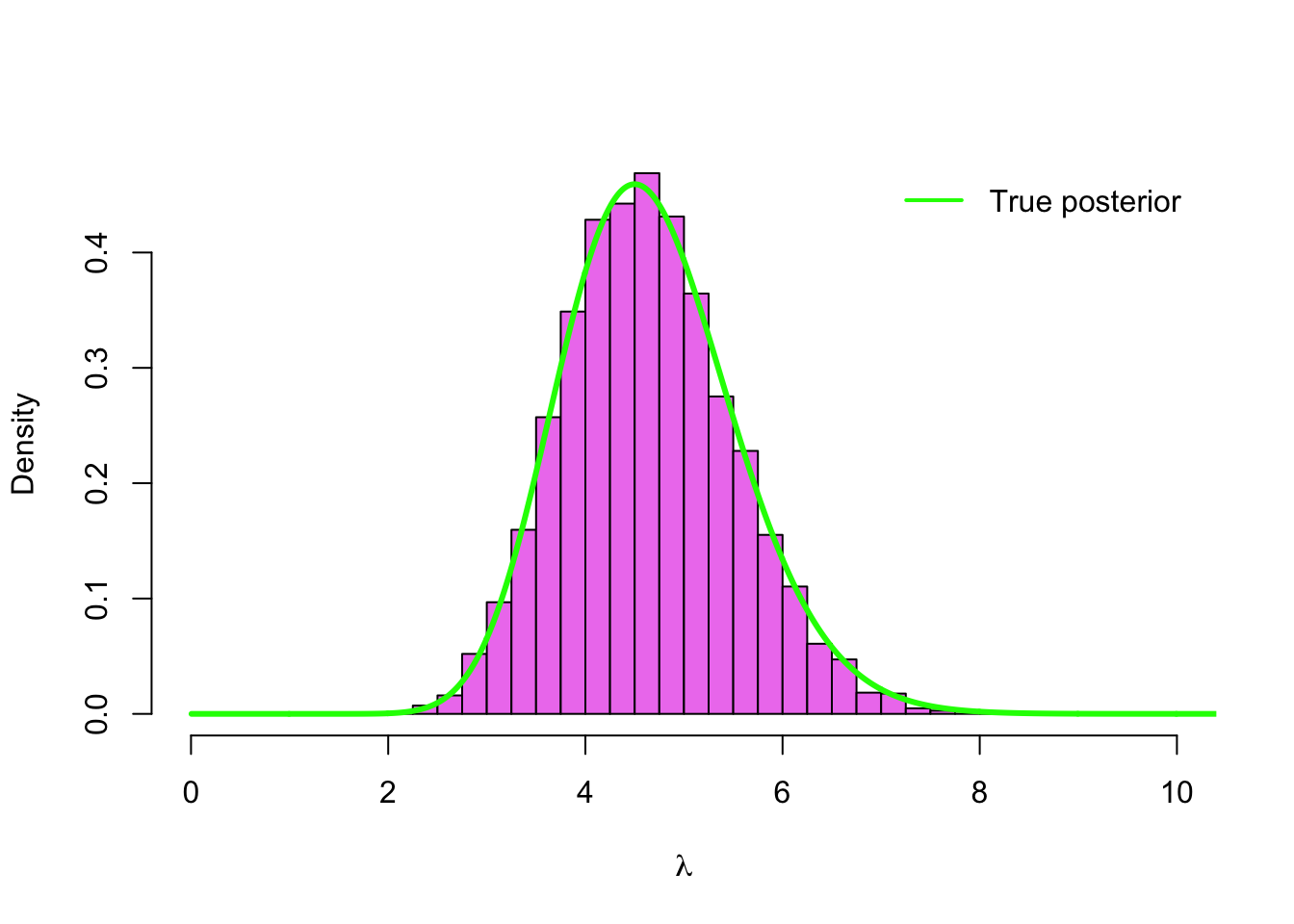
Our simulation seems to have worked correctly! Instead of the histogram we can also compute a smoothed density estimation (with some R magic in the form of density()-function) based on our sample, and verify that it is very close to the true posterior density:
density_sim <- density(lambda_sim)
plot(grid, dgamma(grid, alpha + sum(y), beta + n), type = 'l', col = 'green',
     lwd=3, xlim = c(0,10), bty = 'n', xlab = expression(lambda), ylab = 'Density')
lines(density_sim, type = 'l', col = 'blue', lwd=3 )
legend('topright', legend = c('True posterior', 'Estimated density'),
       col = c('green', 'blue'), lwd = 2, inset = .02, bty = 'n')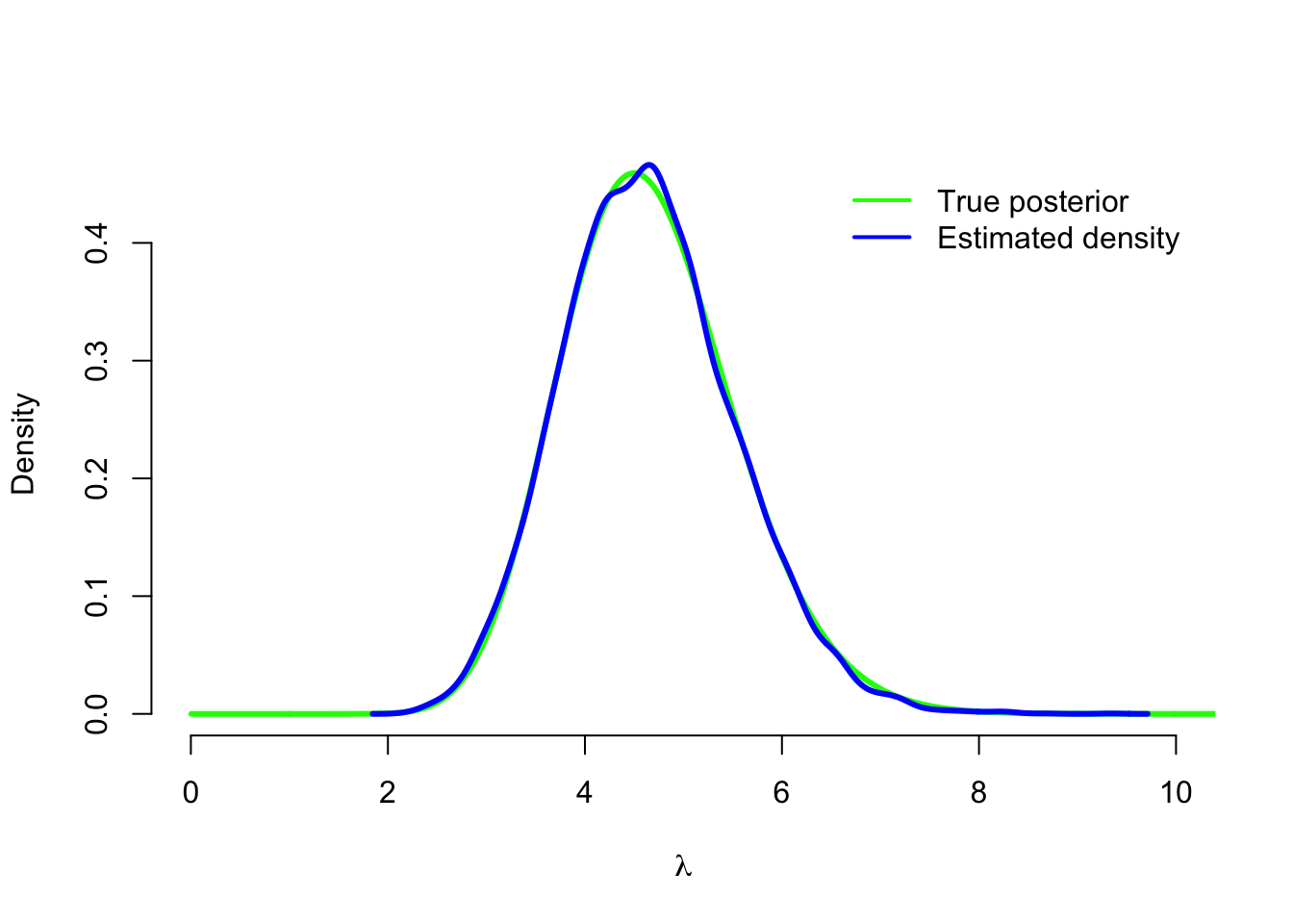
Of course this was not a super interesting example because we already knew a posterior density which we had solved analytically. But now that we are simulating anyway, we don’t actually have to limit our choice of the prior distribution to conjugate priors. So now when we have verified that our simulation algorithm works, let’s try a different prior.
4.1.3 Example : non-conjugate prior for Poisson model
Another popular prior for the Poisson likelihood is a log-normal distribution. If a random variable \(X\) follows a normal distribution \(N(\mu, \sigma^2)\), then \(Y = e^X\) has a log-normal distribution Log-normal\((\mu, \sigma^2)\). And correspondingly, if \(Y \sim \text{Log-normal}(\mu, \sigma^2)\) and \(X = \log Y\), then \(Y \sim N(\mu, \sigma^2)\); hence the name of the distribution. Parameters \(\mu\) and \(\sigma^2\) are not the location and scale parameter of the log-normal distribution, but the location and the scale parameter of the normal distribution you get, when you take a logarithm of the log-normally distributed random variable.
Using a log-normal prior, our model is now: \[ \begin{split} Y_i &\sim \text{Poisson}(\lambda) \quad \text{for all }\,\, i = 1, \dots, n \\ \lambda &\sim \text{Log-normal}(\mu, \sigma^2). \end{split} \] A density function of the log-normal distribution is \[ p(\lambda) = \frac{1}{\lambda\sqrt{2\pi\sigma^2}} e^{-\frac{(\log \lambda - \mu)^2}{2\sigma^2}}, \] and thus we can write the unnormalized posterior density as \[ \begin{split} p(\lambda|\mathbf{y}) &\propto p(\lambda) p(\mathbf{y}|\lambda) \\ &\propto \lambda^{-1} e^{\frac{(\log \lambda - \mu)^2}{2\sigma^2}} \lambda^{\sum_{i=1}^n y_i} e^{-n\lambda} \\ &\propto \lambda^{\sum_{i=1}^n y_i - 1} e^{-n\lambda -\frac{(\log \lambda - \mu)^2}{2\sigma^2}}. \end{split} \] This cannot be normalized into any known probability distribution: the normalizing constant \[ p(\mathbf{y}) = \int p(\lambda) p(\mathbf{y}|\lambda)\,\text{d}\lambda \] is intractable! But this is not a problem, because we know how to simulate from an unormalized posterior distribution. Let’s first define a function3 for the unnormalized posterior:
q <- function(lambda, y, n, mu, sigma_squared) {
  lambda^(sum(y) - 1) * exp(-n * lambda - (log(lambda) - mu)^2 / (2 * sigma_squared))
}
Let’s also set parameters \(\mu = 0\), \(\sigma^2 = 1\) of the prior:
mu <- 0
sigma_squared <- 1
Now we are ready to use our simulation recipe again, and visualize the results:
grid_values <- q(grid, y, n, mu, sigma_squared)
normalized_values <- grid_values / sum(grid_values)
idx_sim <- sample(1:n_grid, n_sim, prob = normalized_values, replace = TRUE)
lambda_sim2 <- grid[idx_sim] + runif(n_sim, -i/2, i/2)

hist(lambda_sim2, col = 'violet', breaks = seq(0,10, by =.25), probability = TRUE,
     main = '', xlab = expression(lambda), xlim = c(0,10), ylim = c(0, 0.5))
lines(grid, dgamma(grid, alpha + sum(y), beta + n), type='l', col='green', lwd=3)
legend('topright', legend = paste0('Gamma(', sum(y) + alpha, ',', n + beta, ')'),
       col = 'green', lwd = 2, inset = .02, bty = 'n')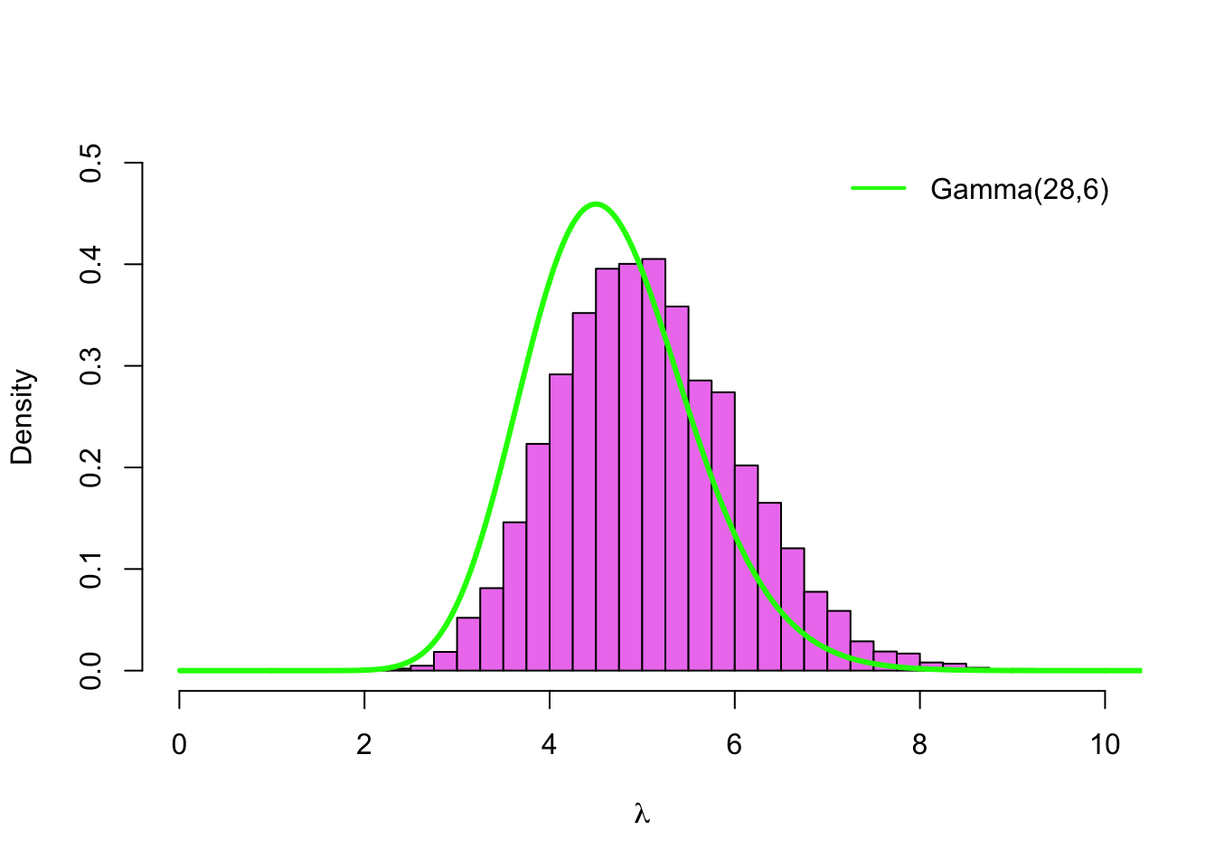
The green line is a density of the posterior with Gamma\((1,1)\)-prior. This time our posterior is concentrated on the slightly higher values. This is because Log-normal\((0,1)\)-distribution has a higher mean \((E\lambda = 1.65)\) and a heavier right tail than the Gamma\((1,1)\)-distribution.
We can also plot estimated posterior density with the log-normal prior, and compare it to the posterior density with the gamma prior:
density_sim <- density(lambda_sim2)
plot(grid, dgamma(grid, alpha + sum(y), beta + n), type = 'l', col = 'green',
     lwd=3, xlim = c(0,10), bty = 'n', xlab = expression(lambda), ylab = 'Density')
lines(density_sim, type = 'l', col = 'blue', lwd=3 )
legend('topright', legend = c(paste0('Gamma(', sum(y) + alpha,
       ',', n + beta, ')'), 'Estimated posterior'), col = c('green', 'blue'),
       lwd = 2, inset = .02, bty = 'n')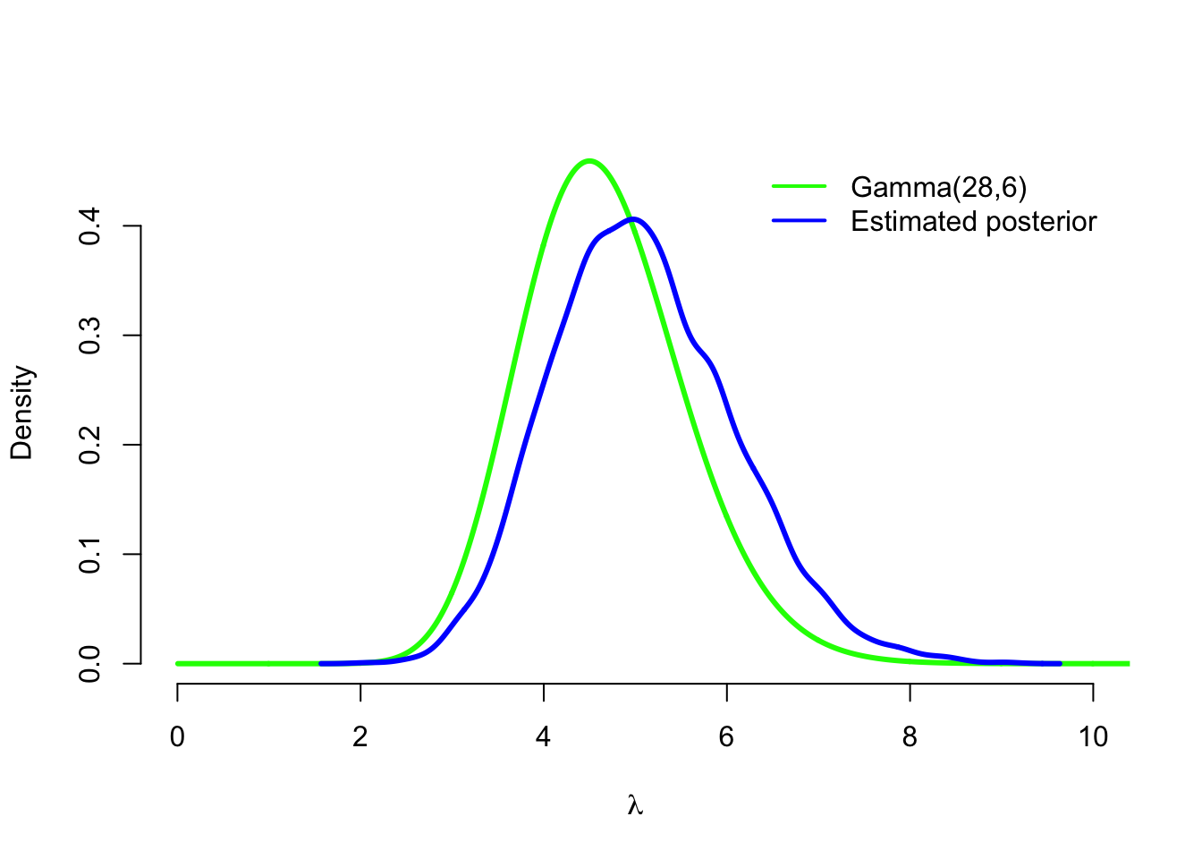
4.2 Monte Carlo integration
In Example 4.1.2 we observed that the empirical posterior density obtained by simulation started to resemble very closely the true posterior density obtained analytically with a high simulation size. This phenomenon can also be utilized to compute summary statistics, such as posterior mean, posterior variance, and credible intervals from the simulated sample.
More generally computing integrals by simulation is known as Monte Carlo integration or Monte Carlo method. It turns on the classical result on a probability theory called a strong law of law numbers4.
4.2.1 Strong law of large numbers (SLL)
Let \(Y_1, Y_2, \dots\) be i.i.d. random variables with an expected value \(\mu := EY_1\) that is finite: \(E|Y_1| < \infty\). Now \[ \frac{1}{n} \sum_{i=1}^n Y_i \rightarrow \mu \] almost surely (a.s.), as \(n\rightarrow \infty\).
Almost sure convergence means that the sequence converges with a probability one: another way to state the result is \[ P\left( \underset{n\rightarrow \infty}{\lim} \frac{1}{n} \sum_{i=1}^n Y_i = \mu \right) = 1. \]
4.2.2 Example of SLL : coinflips
The strong law of law number simply states that the sample mean of i.i.d. random variables converges to an expected value of the distribution with probability one. We intuitively use this result all the time, but the strong law of large numbers states it formally.
Denote by \(Y_1, Y_2, \dots\) a series of coinflips, where \(Y_1 = 1\) means heads and \(Y_1 = 0\) means tails. Assuming a fair coin, \(P(Y_1 = 1) = 1/2\), and thus \(\mu = EY_1 = 1/2\). By a strong law of large numbers the proportion of heads converges to the probability of heads: \[ \frac{1}{n} \sum_{i=1}^n Y_i \overset{\text{a.s.}}{\rightarrow} \frac{1}{2} \] with probability one. Although there exists an infinite number of sequences which do not converge to \(1/2\), such as a sequence of only heads \((1,1, \dots)\), the probability of the set of these sequences is zero.
4.2.3 Example of Monte carlo integration
Let’s revisit Example 4.1.1. Because our simulated values \(\lambda_1, \dots \lambda_S\) are an i.i.d. sample of the posterior distribution, which has a finite expected value, by the strong law of large numbers the posterior mean converges almost surely to this expected value: \[ \frac{1}{S} \sum_{i=1}^S \lambda_i \overset{\text{a.s.}}{\rightarrow} E[\Lambda \,|\, \mathbf{Y} = \mathbf{y}]. \] This means that we can approximate the posterior expectation with the posterior mean: \[ E[\Lambda \,|\, \mathbf{Y} = \mathbf{y}] \approx \frac{1}{S} \sum_{i=1}^S \lambda_i. \] Because we know the posterior expectation \[ E[\Lambda \,|\, \mathbf{Y} = \mathbf{y}] = \frac{\alpha_1}{\beta_1} = \frac{\sum_{i=1}^n Y_i + \alpha}{n + \beta} \] for this example, we can verify that the posterior mean is very close to the true expected value:
alpha_1 <- alpha + sum(y)
beta_1 <- beta + n
alpha_1 / beta_1
## [1] 4.666667mean(lambda_sim)## [1] 4.648235The second moment \(E\lambda^2\) of the posterior distribution also exists, so we can invoke again the strong law of large numbers for the sequence of random variables \(\Lambda_1^2, \Lambda_2^2, \dots\) to approximate the posterior variance: \[ \begin{split} \text{Var}[\Lambda \,|\, \mathbf{Y} = \mathbf{y}] &= E[\Lambda^2 \,|\, \mathbf{Y} = \mathbf{y}] - E[\Lambda \,|\, \mathbf{Y} = \mathbf{y}] \\ &\approx \frac{1}{S} \sum_{i=1}^S \lambda_i^2 - \frac{1}{S} \sum_{i=1}^S \lambda_i \\ &= \frac{1}{S-1} \sum_{i=1}^S (\lambda_i - \overline{\lambda})^2. \end{split} \] Again the empirical variance is very close to the true variance of the posterior distribution:
alpha_1 / beta_1^2 ## [1] 0.7777778var(lambda_sim)## [1] 0.7517682We can also use SLL for the sequence of transformations \(I_{(a,b)}(\Lambda_1), I_{(a,b)}(\Lambda_2), \dots\) of the parameter \(\Lambda\), where \(I_{(a,b)}\) is an indicator function: \[ I_{(a,b)}(x) = \begin{cases} 1 \quad &\text{if} \,\, x \in (a,b), \\ 0 &\text{otherwise}. \end{cases} \] This means that we can approximate the posterior probabilities by the empirical proportions: \[ \begin{split} P(a < \Lambda < b\,|\, \mathbf{Y} = \mathbf{y}) &= E[I_{(a,b)}(\Lambda)\,|\,\mathbf{Y} = \mathbf{y}] \\ &\approx \frac{1}{S} \sum_{i=1}^S I_{(a,b)}(\lambda_i) \\ &= \frac{1}{S} \#\{a < \lambda_i <b\}. \end{split} \] Here \(\#\) marks the number of elements of the set. Let’s demonstrate this by approximating the posterior probabilities \(P(\Lambda > 3 \,|\, \mathbf{Y} = \mathbf{y})\):
pgamma(3, alpha_1, beta_1, lower.tail = FALSE)## [1] 0.9826824mean(lambda_sim > 3)## [1] 0.9811and \(P(4 < \Lambda < 6 \,|\, \mathbf{Y} = \mathbf{y})\):
pgamma(6, alpha_1, beta_1) - pgamma(4, alpha_1, beta_1)## [1] 0.694159mean(lambda_sim > 4 & lambda_sim < 6)## [1] 0.6984Because the empirical distribution function can be used to approximate the cumulative density function \(F_{\Lambda|\mathbf{Y}}\) of the posterior distribution, we can also use the empirical quantiles to estimate the quantiles of the posterior distribution, and thus to approximate equal-tailed credible intervals:
alpha_conf <- 0.05
qgamma(alpha_conf / 2, alpha_1, beta_1) # 0.025 - quantile
## [1] 3.100966quantile(lambda_sim, alpha_conf / 2)## 2.5%
## 3.081615qgamma(1 - alpha_conf / 2, alpha_1, beta_1) # 0.975 - quantiles## [1] 6.547264quantile(lambda_sim, 1 - alpha_conf / 2)## 97.5%
## 6.484451Normally strong law of law numbers is not mentioned explicitly when the empirical quantities are used to approximate expected values, but anyway it is a theoretical result behind these approximations. Also the finiteness of the expected value of the posterior is rarely checked explicitly. However, in the exercises we will have an example of the distribution for which the expected value is infinite.
4.3 Monte Carlo markov chain (MCMC) methods
Our simple grid approximation method worked smoothly, but what would happen if the dimension of the parameter were higher? In our example we set a grid on the interval \((0,10)\) with a grid increment \(i=0.01\), so the grid had 1000 points. If the parameter were two-dimensional, the grid with the same increment over the two-dimensional interval \((0,10) \times (0,10)\) would have million points. And to approximate 3-dimensional parameter with the same grid increment we would need milliard grid points!
Hence, grid approximation quickly becomes infeasible as the dimension of the parameter grows. Rejection and importance sampling have similar problems. This is why for the more complex models sampling is usually done by using Monte Carlo markov chain (MCMC) methods. They are based by iteratively sampling from a Markov chain whose stationary distribution is the target distribution, which in the case of Bayesian computation is most often the posterior distribution \(p(\boldsymbol{\theta}|\mathbf{y})\).
4.3.1 Markov chain
A discrete time Markov chain is a sequence of random variables \(\mathbf{X}_1, \mathbf{X}_2, \dots\), which has a Markov property: \[ P(X_{i+1} = x_{i+1}\,|\, X_{i} = x_{i}, \dots ,X_0 = x_0) = P(X_{i+1} = x_{i+1}\,|\, X_{i} = x_{i}) \] for all \(i = 1, 2, \dots\). This means that any given time the future state \(X_{i+1}\) of the state depends only on the present state \(X_i\) of the chain, and not on the rest of the history.
A state space \(\mathcal{S}\) of the Markov chain is the set of all possible values for these random variables \(X_i\).
4.3.2 MCMC sampling
Simple simulation methods, such as rejection sampling, importance sampling, and grid approximation, which we just demonstrated, generate an i.i.d. sample from the target distribution. However, the components of the sample \(\boldsymbol{\theta_1}, \dots , \boldsymbol{\theta_S}\) generated by the Monte Carlo markov chain methods has a very high autocorrelation: this means that next value \(\boldsymbol{\theta}_{i+1}\) is likely to be somewhere near the current value \(\boldsymbol{\theta}_i\) of the chain. But how does this even work? The trick is that because we generate a large sample, and then use the whole sample to approximate our posterior distribution, the autocorrelation of the single values does not matter.
We already mentioned that the Markov chains used in MCMC methods are designed so that their stationary distribution is the target posterior distribution. But what does the stationary distribution mean? It is simply a distribution \(\pi(x)\) with a following property: if you start the chain from the stattionary distribution so that \(P(X_0 = k) = \pi(k)\) for all \(k\in\mathcal{S}\), then also \(P(X_i = k) = \pi(k)\) for all \(i = 1, 2 \dots\).
This means that once the chain hits its stationary distribution it stays there, and thus the value \(\pi(k)\) is also a long run proportion of the time the chain stays in a state \(k\). And because we defined the chain so that the stationary distribution \(\pi\) is the posterior distribution \(p(\boldsymbol{\theta}|\mathbf{y})\), if the chain moves in it stationary distribution long enough, we get a sample from the posterior!
First iterations of MCMC sampling are usually discarded because the values of the chain before it has converged to the stationary distribution are not representative of the posterior distribution. Exactly how many sampled points are discarded is matter of choice: a very conservative and safe approach is to discard the first half of the iterations. These discarded iterations are called a burn-in period or a warm-up period. Stan discards the warm-up period automatically, so you don’t have to worry about this.
But how do we then know that the chain has converged to its stationary distribution? Actually, in principle this cannot be never known for sure! So we just have to check the model diagnostics (we will examine these more closely later), and check if our results make any sense. Luckily Stan has quite advanced model diagnostics, so it should indicate somehow about the non-convergent chains. An efficient strategy for monitoring the convergence is to run several chains starting from the different initial values in parallel: if they all converge into a similar distribution, it is quite likely that this is the stationary distribution. Stan runs four parallel chains as default.
Markov chains designed so that their stationary distribution is the target posterior distribution, or more generally the implementations of these chains, are called MCMC samplers. The most popular ones are the Gibbs sampler, and the Metropolis-Hastings sampler (actually the Gibbs sampler can also be seen as a special case of the Metropolis-Hasting sampler).
Next we will demonstrate Gibbs sampling with a simple example, so you will get some intuition about how this MCMC sampling business works. However, in this course we will not go into the details about how these samplers work. After this introductory example we will introduce some probabilistic programming tools that have them already implemented, so we don’t have to worry about the technical details, and can concentrate on the statistical inference which this course is all about.
4.3.3 Example of MCMC: Gibbs sampler
The Gibbs sampler is an efficient and popular MCMC sampler which updates components of the parameter vector one at a time. Assume that the parameter vector is multi-dimensional \(\boldsymbol{\theta} = (\theta_1, \dots, \theta_d)\). For each component \(\theta_j\) the Gibbs sampler generates a value from the conditional posterior distribution of this component given all the other components: \[ p(\theta_j \,|\, \boldsymbol{\theta}_{-j}, \mathbf{y}), \] where \(\boldsymbol{\theta}_{-j} = (\theta_1, \dots, \theta_{j-1}, \theta_j, \dots , \theta_d)\).
Let’s demonstrate this with a 2-dimensional example. Assume that we have one observation \((y_1, y_2) = (0,0)\) from the two-dimensional normal distribution \(N(\boldsymbol{\mu}, \boldsymbol{\Sigma}_0)\), where the parameter of interest is a mean vector \(\boldsymbol{\mu} = (\mu_1, \mu_2)\) and the covariance matrix \[ \boldsymbol{\Sigma}_0 = \begin{bmatrix} 1 & \rho \\ \rho & 1 \end{bmatrix} \] is assumed as a known constant matrix. Assume that the covariance is \(\rho = -0.7\). Further assume that we are using an improper uniform prior \(p(\boldsymbol{\mu}) \propto 1\) for parameter \(\boldsymbol{\mu}\). Now the posterior is (do not care about the inference of the posterior right now; we will consider posterior inference for the multi-dimensional parameter on next week) a 2-dimensional normal distribution \(N(\boldsymbol{\mu}, \boldsymbol{\Sigma}_0)\).
Of course we could generate a sample from this normal distribution using a library implementation of the multinormal distribution, but let’s write a Gibbs sampler to demonstrate MCMC methods in practice.
From the properties of the multinormal distribution we get the conditional posterior distributions of \(\mu_1\) given \(\mu_2\), and \(\mu_2\) given \(\mu_1\): \[ \begin{split} \mu_1 \,|\,\mu_2, \mathbf{Y} &\sim N(y_1 + \rho(\mu_2 - y_2),\, 1 - \rho^2) \\ \mu_2 \,|\,\mu_1, \mathbf{Y} &\sim N(y_2 + \rho(\mu_1 - y_1),\, 1 - \rho^2). \end{split} \] To implement a Gibbs sampler, let’s set the parameter and observation values and define these conditional posterior distributions:
y <- c(0,0)
rho <- -0.7

mu1_update <- function(y, rho, mu2) rnorm(1, y[1] + rho * (mu2-y[2]), sqrt(1-rho^2))
mu2_update <- function(y, rho, mu1) rnorm(1, y[2] + rho * (mu1-y[1]), sqrt(1-rho^2))
Note that in R the normal distribution is parametrized with standard devation, not variance, so that the parameter is \((\mu, \sigma)\) instead of the usual parameter \((\mu, \sigma^2)\). A classical R mistake is to give for dnorm or rnorm the variance instead of the standard deviation, and then wonder why the results look strange… I have done this many times. Anyway, this is why we take the square root of the variance when we plug it into the formula.
Then we will set an initial value \((2,2)\) for \(\boldsymbol{\mu}\), and start sampling:
n_sim <- 1000
mu1 <- mu2 <- numeric(n_sim)
mu1[1] <- 2
mu2[1] <- 2

for(i in 2:n_sim) {
  mu1[i] <- mu1_update(y, rho, mu2[i-1])
  mu2[i] <- mu2_update(y, rho, mu1[i])
}
This was all that was required to implement a Gibbs sampler! Let’s examine the trace of the sampler after 10, 100, and 1000 simulation rounds:
draw_gibbs <- function(mu1, mu2, S, points = FALSE) {
  plot(mu1[1], mu2[1], pch = 4, lwd = 2, xlim = c(-4,4), ylim = c(-4,4), asp = 1,
       xlab = expression(mu[1]), ylab = expression(mu[2]), bty = 'n', col = 'darkred')
  for(j in 2:S) {
    lines(c(mu1[j-1], mu1[j]), c(mu2[j-1], mu2[j-1]), type = 'l', col = 'darkred')
    lines(c(mu1[j], mu1[j]), c(mu2[j-1], mu2[j]), type = 'l', col = 'darkred')
    if(points) points(mu1[j], mu2[j], pch = 16, col = 'darkred')
  }
  text(x = -3, y = -2.5, paste0('S=', S), cex = 1.75)
}

draw_sample <- function(mu1, mu2, ...) {
  plot(mu1, mu2, pch = 16, col = 'darkgreen',
       xlim = c(-4,4), ylim = c(-4,4), asp = 1, xlab = expression(mu[1]),
       ylab = expression(mu[2]), bty = 'n', ...)
}

par(mfrow = c(2,2), mar = c(2,2,4,4))
draw_gibbs(mu1, mu2, 10, points = TRUE)
draw_gibbs(mu1, mu2, 100)
draw_gibbs(mu1, mu2, n_sim)
draw_sample(mu1[10:length(mu1)], mu2[10:length(mu2)], cex = 0.7)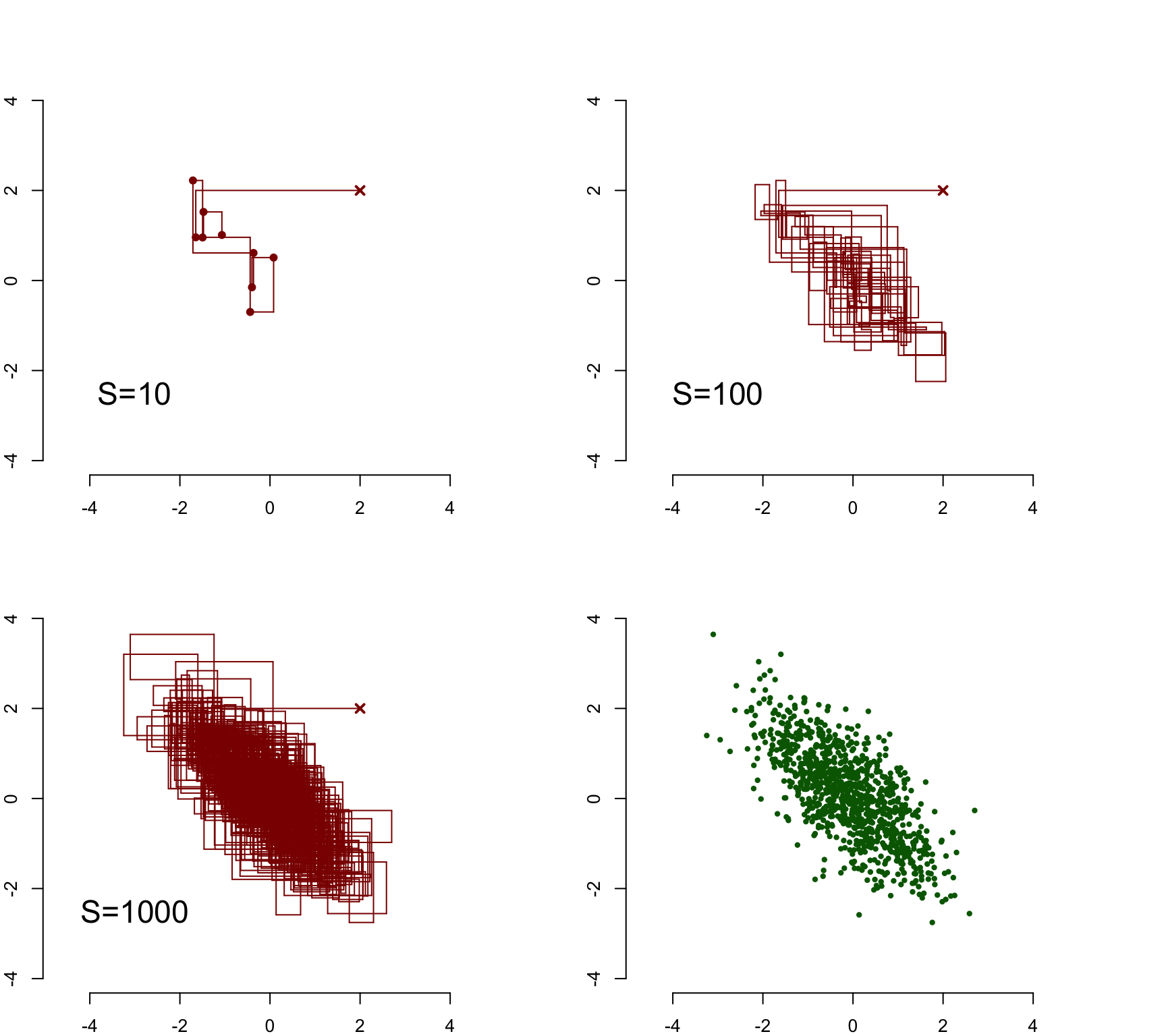
Although the initial value was away from the center of the probability mass of the distribution, the sampler moved quickly to the dense area of the distribution, and after this seemed to explore it efficiently. These trace plots also illustrate the autocorrelation of the sample: subsequent samples (marked explicitly into the first plot with \(S=10\)) tend to be close to another.
The last plot contains the sampled points (with a burn-in period of 10 points discarded): although the sample is autocorrelated, this does not matter for the final results. In fact, our MCMC sample is indistinguishable from the i.i.d. sample from the true posterior distribution:
Sigma <- matrix(c(1, rho, rho, 1), ncol = 2)
X <- MASS::mvrnorm(n_sim, y, Sigma)

par(mfrow = c(1,2), mar = c(2,2,4,4))
draw_sample(mu1[10:length(mu1)], mu2[10:length(mu2)], cex = 0.5, main = 'MCMC')
draw_sample(X[ ,1], X[ ,2], cex = 0.5, main ='i.i.d.')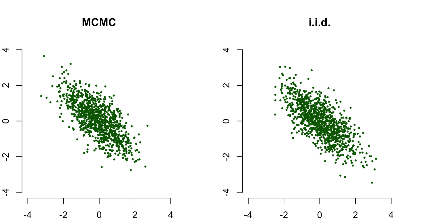
4.4 Probabilistic programming
Although easy in our introductory example, deriving and testing the samplers quickly becomes very time-consuming when models become more complicated. It may take several weeks worth of effort from a stastician to derive an efficient sampler for the new model. This has been one of the main reasons why it has took so long to adapt Bayesian methods into the mainstream statistical practice, although the main principles of Bayesian statistics are even older than the ones of frequentist statistics, which originated in the beginning of the last century. Another, and in the past of course more restricting, reason has been a lack of computational power required to do efficient sampling.
But nowadays computers are fast enough, and luckily also the human effort required has diminished significantly : probabilistic programming systems, which have multi-purpose samplers that can be used to generate a sample of the posterior of the very large array of models, so that we don’t have to write a specific sampler for each different model.
Probabilistic programming means basicly automatic inference of (often, but not necessarily, Bayesian) statistical models. In principle, the only thing the user has to do is to specify the statistical model in a high-level modelling language, and the probabilistic programming system takes care of the sampling. Using these systems has an advantage that they abstract most of the computational details from us (at least when the sampling works…), so that we can concentrate on building the statistical model instead of implementing the sampler.
One of the pioneers of probabilistic programming tools5 was BUGS (Bayesian inference Using Gibbs Sampling). As the abbreviation hints, it used Gibbs samplers to approximate posterior, and was widely used on the fields requiring applied statistics (or at least by those who used Bayesian methodology on those fields).
However, in the recent years much more powerful probabilistic programming tools have emerged. In part this is because of the development on the Hamiltonian Monte Carlo (HMC) methods, which allows sampling from a much more general class of models than the Gibbs samplers. The most well-known of these new tools are Stan, PyMC3 and Edward.
Next we are going to get familiar with probabilistic programming by using Stan, and more specifically RStan, which is its R interface. The Stan library itself is written in C++, and in addition to R, it has an interface also for Python (PyStan) and some other high-level languages.
Installing RStan requires little more tuning than installing a normal R package. Detailed instructions for installing RStan for your operating systems can be found from: RStan-Getting-Started. That being said, installing RStan for Linux or MacOS may also work by just running the following line in R:
install.packages("rstan", repos = "https://cloud.r-project.org/", dependencies=TRUE)However, your mileage may vary; and following the official instructions is anyway recommended to optimize the compiling and running speed of Stan models.
4.4.1 Minimal Stan-example : model declaration
Now that you have installed Stan, all the hard work is done: fortunately using it fun and easy! When trying new software, I like to run a minimal “Hello World!”-example just to check that everything is set up and working correctly. So as a “Stan - Hello world!” - example, let’s revisit Example 2.1.1 (Poisson sampling distribution with gamma prior) again, and this time use Stan to simulate from the posterior.
Stan models are specified using a high-level modeling language whose syntax resembles R syntax. Models are written into their own .stan-files, which Stan first translates into C++ code and then compiles. Let’s start writing our model into a new file, which we can name for example as poisson.stan.
A stan model consists of named blocks which are written inside the curly brackets. In principle all the blocks are optional, but three necessary blocks to specify a non-trivial probability model are data, parameters, and model.
First we need to declare the variables for the input data of our model into the data-block:
data {
  int<lower=0> n;
  int<lower=0> y[n];
}
We declared a sample size n as a non-negative integer, and y as a vector of non-negative integers having n components. Note that unlike in R syntax, we had to specify data types of the variables we are declaring; and in addition to specifying our variables as integers, we also constrained them to be non-negative integers with the speficier lower=0. We could have also constrained our variable into a certain interval: for example we could declare the observation y from the binomial distribution Bin\((n, \theta)\), which is constrained into the interval \((0,n)\), as follows:
int<lower=0,upper=n> y;Constraining the variables correctly (so that they are constrained to the support of their distribution6) is especially important when declaring the parameters, because Stan uses these constraints when sampling.
Notice also that unlike in R or Python, but like in C++ or Java, each line ends with a semicolon. Omitting it is a syntax error.
Next we declare the parameters of the model in the parameters-block:
parameters {
  real<lower=0> lambda;
}
Parameter of the Poisson\((\lambda)\) distribution is a real number, so we declare its type as real. Note that we do not declare the hyperparameters of the prior Gamma\((\alpha, \beta)\)-distribution in the parameters-block, because we consider them as fixed constants (here \(\alpha = 1\), \(\beta = 1\)), not as random variables like \(\lambda\).
Finally, we specify our probability model in the model-block:
model {
  lambda ~ gamma(1,1);
  y ~ poisson(lambda);
}
Compare this to our usual model declaration: \[ \begin{split} Y_i &\sim \text{Poisson}(\lambda) \quad \text{for all}\,\, i = 1, \dots , n \\ \lambda &\sim \text{Gamma}(1,1) \end{split} \] Look pretty similar, right? Stan declaration is even a bit simpler, because Stan supports vectorization: a statement
y ~ poisson(lambda);for the vector y means that each component of this vector follows Poisson\((\lambda)\)-distribution. We could have also used a more explicit and verbose form:
for(i in 1:n)
  y[i] ~ poisson(lambda);
A syntax of the for loop is similar to R. The body of the loop is enclosed in the curly brackets; if it consists only of one line, as above, these curly brackets can be omitted.
Our first two blocks consist of only variable declarations. The model-block is different: it contains statements. The statements of the form
y ~ poisson(lambda);are called sampling statements. They simply tell Stan which probability distribution our variables follow; these sampling statements are used to implement the sampler for the model.
Stan supports most of the well-known distributions, and it is also possible to define own probability distributions by supplying its log-density function. A full list of the available distributions (and tons of other information) can be found from Stan reference manual.
So our full stan model, which we save into the file poisson.stan, is:
data {
  int<lower=0> n;
  int<lower=0> y[n];
}

parameters {
  real<lower=0> lambda;
}

model {
  lambda ~ gamma(1,1);
  y ~ poisson(lambda);
}
4.4.2 Minimal Stan-example : sampling
We have now specified our model and are ready to generate a sample from the posterior. But let’s first generate our old data set \(\mathbf{y}\):
lambda_true <- 3
n_sample <- 5
set.seed(111111)
(y <- rpois(n, lambda_true))
## [1] 4 3 11 3 6Then we wrap our observations and sample size into a list, which has components with the names corresponding to the variables declared in data-block of the Stan model:
poisson_dat <- list(y = y, n = n_sample)We have not yet loaded a package RStan, so let’s do it now:
library(rstan)## Loading required package: ggplot2## Loading required package: StanHeaders## rstan (Version 2.18.2, GitRev: 2e1f913d3ca3)## For execution on a local, multicore CPU with excess RAM we recommend calling
## options(mc.cores = parallel::detectCores()).
## To avoid recompilation of unchanged Stan programs, we recommend calling
## rstan_options(auto_write = TRUE)Hmm, it recommends to run some code, so let’s do it:
rstan_options(auto_write = TRUE)
options(mc.cores = parallel::detectCores())
The first line allows saving the compiled model to the hard disk, so it saves time because the model does not has to be recompiled every time it is used. The second line allows Stan to run several Markov chains in parallel, which also saves time.
Now we are finally ready for the actual sampling. The sampling is done via stan-function. The following code works if the poisson.stan-file that contains the model is in your working directory:
fit <- stan(file = 'poisson.stan', data = poisson_dat)
# I cut the compiler and sampler messages from here to make this look more clean
Function stan first compiles the model, then draws a sample from the posterior, and finally returns the sampled values as stanfit object. Let’s print the summary of the returned stanfit-object:
fit## Inference for Stan model: poisson.
## 4 chains, each with iter=2000; warmup=1000; thin=1;
## post-warmup draws per chain=1000, total post-warmup draws=4000.
##
## mean se_mean sd 2.5% 25% 50% 75% 97.5% n_eff Rhat
## lambda 4.71 0.02 0.88 3.14 4.10 4.66 5.25 6.54 1726 1
## lp__ 14.64 0.02 0.71 12.69 14.49 14.92 15.09 15.13 2033 1
##
## Samples were drawn using NUTS(diag_e) at Wed Mar 13 10:37:47 2019.
## For each parameter, n_eff is a crude measure of effective sample size,
## and Rhat is the potential scale reduction factor on split chains (at
## convergence, Rhat=1).Stan runs as default 4 chains for 2000 iterations each, and it discards first half of the iterations as the warm-up period. So the default sample size is 4000, as shown above. Stan reports mean, median and 50% and 95% equal-tailed credible interval for our parameters of interest, in this case \(\lambda\).
You can also run function stan without specifying the argument data. In case you omit this argument, Stan tries to find the input data (variables y and n) from the global R enviroment. With our model this would probably fail, because we have defined a sample size using the variable n_sample, not the variable n. Or then it would be pick some n we have defined earlier in our code, which may or may not be correct. So it is much more clear and less error-prone to specify the input data explicitly as a list.
4.4.3 Minimal Stan example : illustrating the results
We can draw a boxplot of the simulated posterior distribution of the parameter \(\lambda\) simply as:
plot(fit)## ci_level: 0.8 (80% intervals)## outer_level: 0.95 (95% intervals)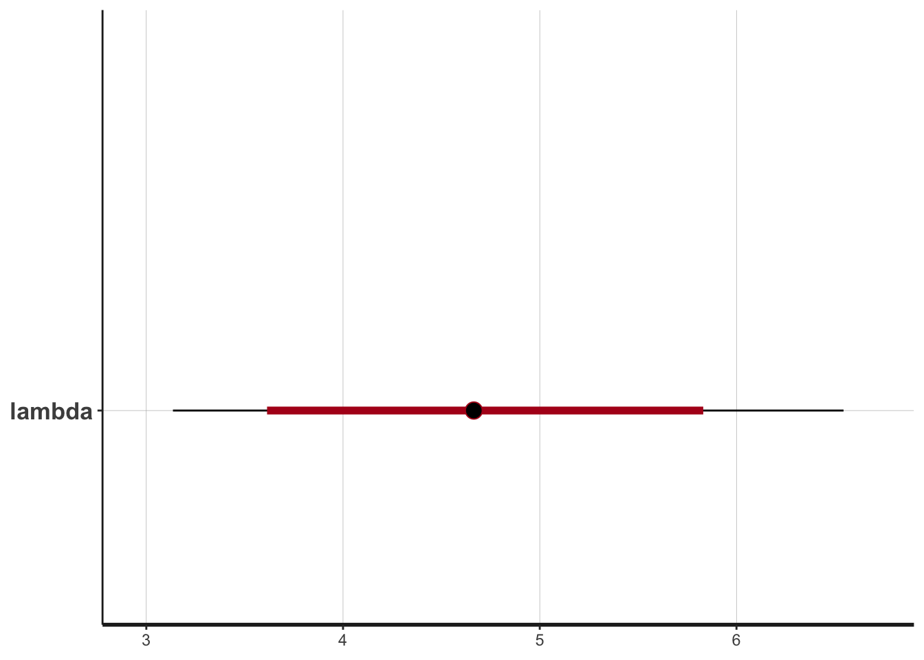
Compare this to Figure 3.1: 95% CI estimated from the posterior lies slightly above the true parameter value (\(\lambda=3\)) of the generating distribution, as does the 95% CI computed based on the exact posterior distribution.
The simulated values can be extracted from the stanfit-object with extract-function:
sim <- extract(fit, permuted = TRUE)
str(sim)
## List of 2
## $ lambda: num [1:4000(1d)] 5.73 5.58 6.09 3.9 4.03 ...
## ..- attr(*, "dimnames")=List of 1
## .. ..$ iterations: NULL
## $ lp__ : num [1:4000(1d)] 14.5 14.7 14 14.7 14.8 ...
## ..- attr(*, "dimnames")=List of 1
## .. ..$ iterations: NULLThese simulated values can be used like any sample from the posterior distribution. We can for example draw a histogram of the sample:
hist(sim$lambda, breaks = 50, col = 'violet', probability = TRUE,
     main = paste0('S = ', length(sim$lambda)), xlab = expression(lambda))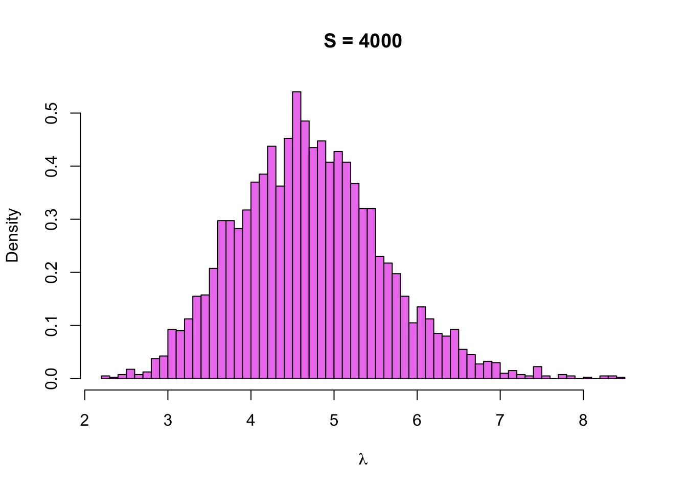
Hmm, it looks a little bit jagged, so maybe we should increase the sample size. Function stan has arguments chains and iter, which can be used to specify the sample size. Let’s set iterations to 20000, which means that we should get a sample of \(4 \cdot 20000 / 2\) = 40000 points:
fit <- stan(file = 'poisson.stan', data = poisson_dat, iter = 20000, chains = 4)
sim <- extract(fit, permuted = TRUE)
str(sim$lambda)
## num [1:40000(1d)] 3.35 5.92 5.08 4.78 5.92 ...
## - attr(*, "dimnames")=List of 1
## ..$ iterations: NULLNotice how everything worked much faster this time (at least if we have ran the line rstan_options(auto_write = TRUE)), even though the sample size of the simulation was 10 times higher? This is because Stan does not have to compile the model again; for this simple model compiling the model takes actually much longer than sampling from it (unless your simulation sample size is astronomic).
Let’s draw a histogram of the sample with the density function of the true posterior \(\text{Gamma}\,(\sum_{i=1}^n y_i + 1, n + 1)\) on top of it:
x <- seq(0,10, by = .01)
hist(sim$lambda, breaks = 50, col = 'violet', probability = TRUE,
     main = paste('S =', length(sim$lambda)), xlab = expression(lambda))
lines(x, dgamma(x, sum(y) + 1, n_sample + 1), col = 'blue', type = 'l', lwd = 2)
legend('topright', legend = 'True posterior', lwd = 2, col = 'blue',
       inset = 0.01, bty = 'n')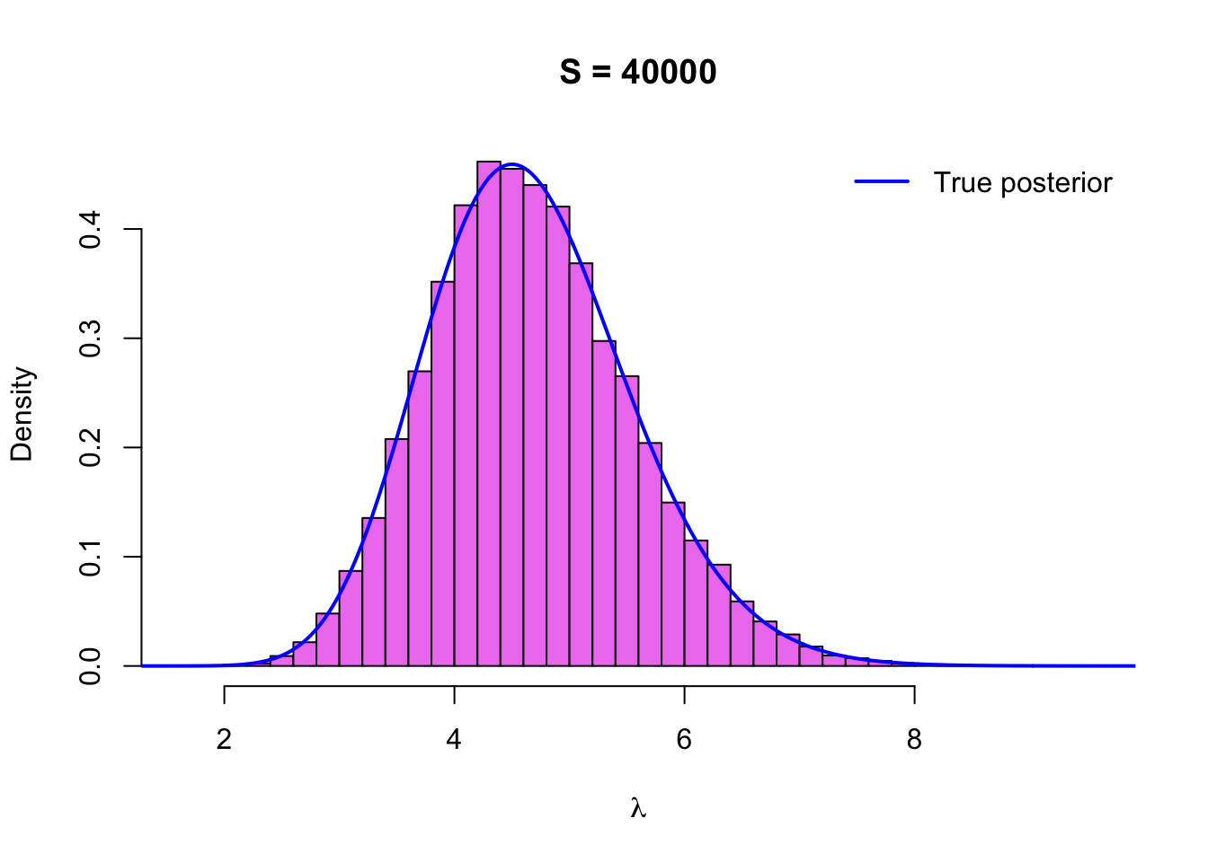
The histogram looks now smoother as we expected, and it also seems to match the density of the true posterior very well, so everything seems to be working as it should.
4.4.4 Minimal Stan-example: changing the prior
To make our minimal Stan example not so minimal anymore, let’s change the prior of our model to the Log-normal distribution, so that the new model is: \[ \begin{split} Y_i &\sim \text{Poisson}(\lambda) \quad \text{for all} \,\, i = 1, \dots , n \\ \lambda &\sim \text{Log-normal}(\mu, \sigma^2). \end{split} \] Let’s also use hyperparameters \(\mu = 0, \sigma^2 = 1\). To declare this model in Stan modelling language, the only thing we have to change in our previous declaration is to change the prior distribution for the parameter \(\lambda\):
data {
  int<lower=0> n;
  int<lower=0> y[n];
}

parameters {
  real<lower=0> lambda;
}

model {
  lambda ~ lognormal(0,1);
  y ~ poisson(lambda);
}
Let’s save this model into the file poisson_lognormal.stan, and generate a sample from it:
fit2 <- stan('poisson_lognormal.stan', iter = 20000, chains = 4)Now we can draw a histogram of the sample, and compare it to the posterior with the \(\text{Gamma}(1,1)\)-prior and the estimated density of the posterior with the same \(\text{Log-normal}(0,1)\)-prior, which we simulated via grid approximation in Example 4.1.2:
sim2 <- extract(fit2, permuted = TRUE)
x <- seq(0,10, by = .01)
hist(sim2$lambda, breaks = 50, col = 'violet', probability = TRUE,
     xlab = expression(tilde(y)), ylim = c(0, 0.45),
     main = 'Posterior density')
lines(x, dgamma(x, sum(y) + alpha, n_sample + beta), col = 'blue', type = 'l', lwd = 2)
lines(density_sim, type = 'l', col = 'green', lwd=3 )
legend('topright', legend = c('with Gamma prior', 'with Log-normal prior'),
       col = c('blue', 'green'), lwd = 2, bty = 'n')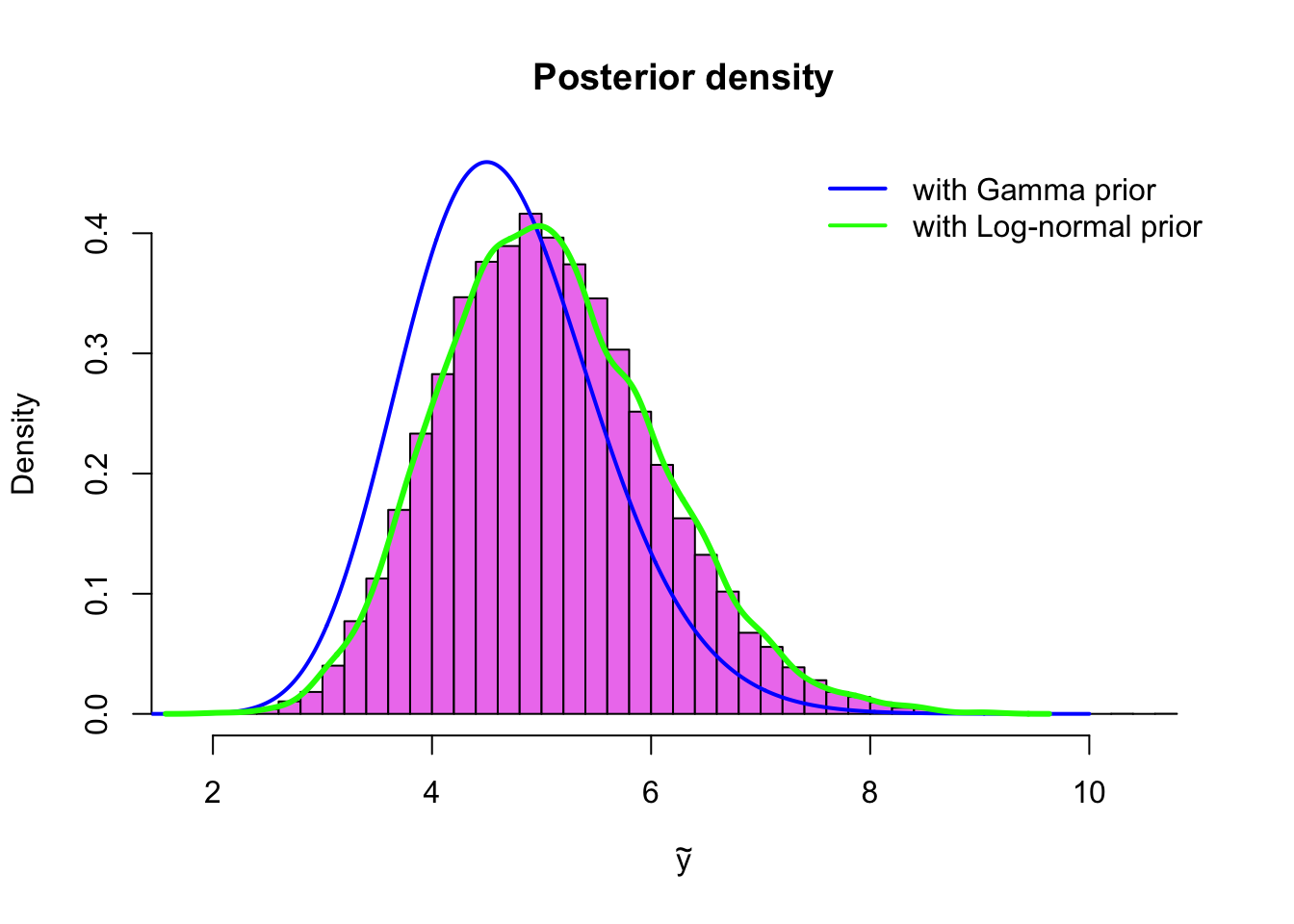
With Stan changing the prior distribution is very convenient. This makes it easy to try different prior distributions to see how sensitive your posterior inference is to the choice of prior distribution. If your posterior inferences are robust with respect to the choice of prior, that is, they do not change very much if you change your prior (assuming of course that the priors are reasonably non-informative), this is a good thing. This is called sensitivity analysis.
4.5 Sampling from posterior predictive distribution
We have demonstrated sampling from the posterior distribution, but how about the posterior predictive distribution? Turns out that this is super easy once we have a sample from the posterior distribution!
Let’s assume for simplicity that we want to predict probabilities for the new observation \(\tilde{Y}\) from the same process as the original observations \(\mathbf{Y} = (Y_1, \dots, Y_n)\) (for many new observations the posterior predictive distribution is same for every observation if they are i.i.d.).
Assume that we have generated the sample \(\boldsymbol{\theta}_1, \dots , \boldsymbol{\theta}_S\) from the posterior distribution \(p(\mathbf{y}|\boldsymbol{\theta})\). Now the simulation recipe to generate the sample \(\tilde{Y}_1, \dots, \tilde{Y}_S\) from the posterior distribution is simply:
- For all \(s = 1, \dots, S\):
- Draw \(\tilde{Y}_s \sim p(\tilde{y}| \boldsymbol{\theta}_s)\)
So for each value of the parameter we sampled from the posterior distribution, we draw a new observation \(\tilde{Y}\) from its sampling distribution into which we have plucked the sampled parameter value.
The empirical distribution of this sample can be used to approximate the posterior predicitive distribution, which is a sampling distribution averaged (with weights given by the posterior distribution) over the possible parameter values: \[ p(\tilde{y}|\mathbf{y}) = \int p(\tilde{y}|\boldsymbol{\theta}) p(\boldsymbol{\theta}|\mathbf{y}) \,\text{d}\boldsymbol{\theta} \]
Notice how this is different from plugging a single point estimate \(\hat{\boldsymbol{\theta}}\), such as the posterior mean or the maximum likelihood estimate to the sampling distribution for the new observation, that is, using \(p(\tilde{y}|\hat{\boldsymbol{\theta}})\) to predict the probabilities for the new values.
In practice, we can take a kernel density estimate of our simulated sample \(\tilde{y}_1, \dots, \tilde{y}_S\), and use it to approximate the density of the posterior predictive distribution \((\tilde{y}|\mathbf{y})\). Or if the sampling distribution of \(\tilde{Y}\) is discrete, then we can simply just normalize the counts into a probability distribution, as we will do in the following example.
4.5.1 Example : sampling from the posterior predictive distribution
Let’s revisit our first Stan example (Example 4.4.1). Assume that we want a predictive distribution \(p(\tilde{y}|\mathbf{y})\) for the new observation \(\tilde{Y} \sim \text{Poisson}(\lambda)\) given the old observations \(Y_1, \dots, Y_n\).
Now that we have generated the sample \(\lambda_1, \dots, \lambda_S\) from the posterior distribution, we can generate the sample \(\tilde{y}_1, \dots \tilde{y}_S\) from the posterior predictive distribution simply as:
y_pred <- rpois(length(lambda_sim), lambda_sim)Because the sampling distribution of \(\tilde{Y}\) is discrete, we can approximate the posterior predictive distribution by normalising the counts of our simulated sample into a probability distribution. We have solved the true posterior predictive distribution \[ \tilde{Y} \,|\, \mathbf{Y} \sim \text{Neg-bin}\left(\sum_{i=1}^n y_i + \alpha, \, \frac{n + \beta}{n + \beta + 1}\right) \] for this model in Example 2.1.2, so let’s draw both our approximation and the true distribution to verify that they closely match each other:
y_pred <- rpois(length(sim$lambda), sim$lambda)
post_pred <- table(y_pred) / sum(table(y_pred))
plot(post_pred, col = 'violet', lwd = 2, ylab = 'Probability',
     xlab = expression(tilde(y)), bty = 'n')
x <- 0:20
lines(x, dnbinom(x, sum(y) + alpha,  (n_sample + beta) / (n_sample + beta + 1)),
      col = 'green', type = 'b', lwd = 2)
legend('topright', legend = c('Simulated posterior predictive',
       'True posterior predictive'), col = c('violet', 'green'),
       lwd = 2, bty = 'n', inset = 0.01)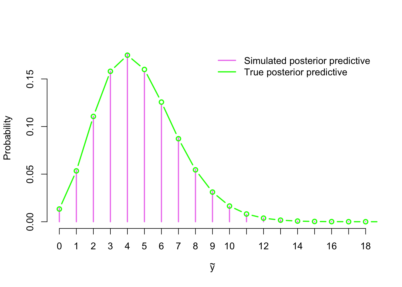
Normally we would compute with the logarithms, which means using values of the function \(\log q(\lambda; \mathbf{y})\) instead of \(q(\lambda;\mathbf{y})\), and exponentiate as late as possible to avoid over- and underflows and other numerical problems. However, let’s not complicate things unnecessarily in this introductory example.↩
There are several versions of law of large numbers with different assumptions; the version introduced here was proved by Kolmogorov in 1930s.↩
Although BUGS was an early example of probabilistic programming, the nomer probabilistic programming is quite recent. BUGS project was originated in 1989, so it is much older than this term.↩
Support of the continuous probability distribution is a set where its density is positive.↩