Bayesian Inference 2019
2019-03-13
Chapter 1 Introduction
1.1 Motivating example : thumbtack tossing
A classical toy example of the random experiment in probability calculus is coin tossing. But this is a little bit boring example, since we know (at least if the coin is fair) a priori that the probability of both heads and tails is very close to \(0.5\).
Instead, let’s consider a slightly more interesting toy example: thumbtack tossing. If we define the success as a thumbtack landing with its point up, we can only have a vague guess about the success probability before conducting the experiment.
Let’s toss a thumptack \(n\) times, and count the number of times it lands with its point up; denote this quantity as \(y\). We are interested in deducing the true success probability \(\theta\).
Probably our first intuition is just to use the proportion of successes \(y/n\) as an estimate of the true success probability \(\theta\). But consider an outcome where you tossed the thumptack \(n=3\) times, and each time the thumbtack landed point down; this means that your observed value is \(y=0\). Would it be sensible to conclude that the true success probability in this is \(\theta = y/n = 0/3 = 0\)? It clearly makes no sense to conclude that the true underlying success probability \(\theta\) is equal to the observed proportion \(y/n\).
Also if we toss the thumbtack \(n=3000\) times and observe the zero successes, the proportion of successes is also \(y/n = 0\), but now it would make much more sense conclude that thumbtack landing point up is actually impossible, or at least a very rare event.
So in addition to the most probable value of \(\theta\) we also need to measure the uncertainty of our estimates. Finding the most likely parameter values, and quantifying our uncertainty about them is called statistical inference.
1.1.1 Modelling thumbtack tossing
To generate some real world data I threw a thumbtack \(N = 30\) times. It landed point up \(16\) times, and point down \(14\) times; this means we observed a data set \(y = 16\).
Let’s define a proper statistical model to quantify our uncertainty of the true probability of the thumptack landing point up. We can consider an observed proportion of the successes \(y\) as a realization of random variable \(Y\). As we remember from the probability calculus course, a repeated random experiment with constant success probability, binary outcome and independent repetitions is modelled with binomial distribution: \[ Y \sim \text{Bin}(n,\theta), \,\,\, 0 < \theta < 1. \] This means that random variable \(Y\) follows a binomial distribution with a (fixed) sample size \(n\) and a success probability \(\theta\). Unknown quantities in the model, such as \(\theta\) here, are called parameters of the model.
The functional form of the probability mass function (pmf) of \(Y\): \[ f(y; n, \theta) = \binom{n}{y} \theta^y (1-\theta)^{n-y} \] is fixed, and the value the parameter \(\theta\) determines what it looks like. Let’s draw some pmf:s of \(Y\) with a fixed sample size \(N=30\), and different parameter values:
par(mar = c(4, 4, .1, .1))
n <- 30
y <- 0:30
theta <- c(3, 10, 25) / n
plot(y, dbinom(y, size = n, prob = theta[1]), lwd = 2, col = 'blue', type ='b',
     ylab = 'P(Y=y)')
lines(y, dbinom(y, size = n, prob = theta[2]), lwd = 2, col = 'green', type ='b')
lines(y, dbinom(y, size = n, prob = theta[3]), lwd = 2, col = 'red', type ='b')
legend('top', inset = .02, legend = c('Bin(30, 1/10)', 'Bin(30, 1/3)', 'Bin(30, 5/6)'),
       col = c('blue', 'green', 'red'), lwd = 2)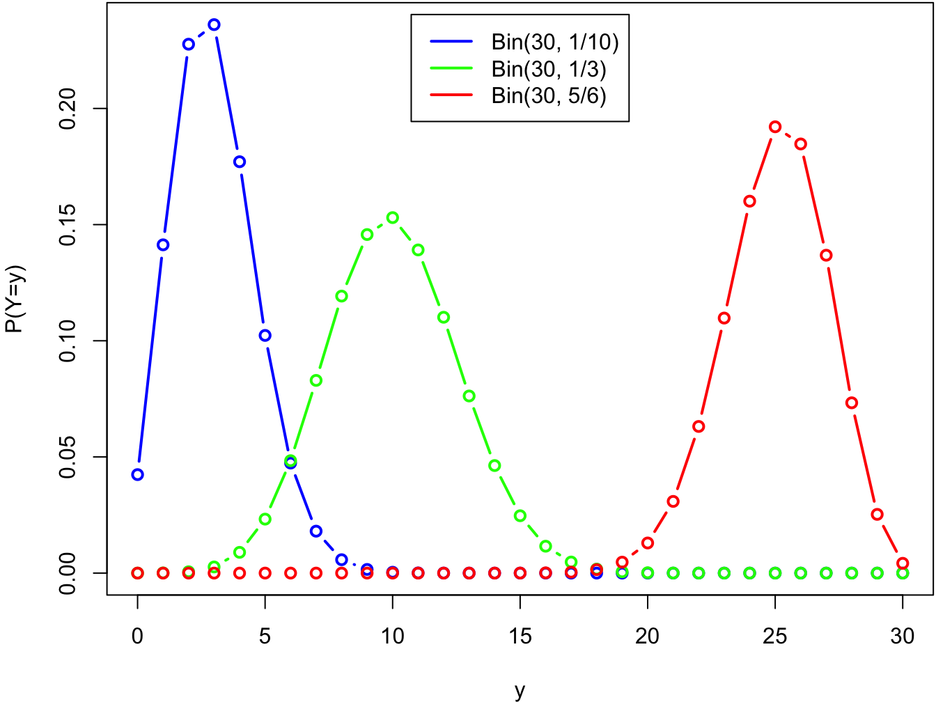
1.1.2 Frequentist thumbtack tossing
In classical (sometimes called frequentist) statistics we consider the likelihood function \(L(\theta;y)\); this is just a pmf/pdf of the observations considered as a function of parameter \(\theta\): \[ \theta \mapsto f(y;\theta). \] Then we can find the most likely value of the parameter by maximizing the likelihood function (normally we actually maximize the natural logarithm of the likelihood function often called the log-likelihood, \(l(\theta;y) = \log L(\theta;y)\), which is computationally more convenient) w.r.t. parameter \(\theta\). This means that we find the parameter value, which has a highest probability of producing this particular data set. This parameter value \(\hat{\theta}\), which maximizes the likelihood function is called a maximum likelihood estimate: \[ \hat{\theta}(y) = \underset{\theta}{\text{argmax}} \,\, L(\theta; y). \] The maximum likelihood estimate is the most likely value of the parameter given the data.
Let’s derive the maximum likelihood estimate for our binomial model. Because logarithm is a monotonusly increasing function, the global maximum point of the log-likelihood maximizes also the likelihood function. Log-likelihood for this model is: \[ l(\theta; y) = \log f(y;\theta) \propto \log(\theta^y(1-\theta)^{n-y}) = y\log\theta + (n-y)\log(1-\theta) \] We dropped the normalizing constant \(\binom{n}{y}\) from the likelihood function because it is a constant w.r.t. parameter \(\theta\), and thus has no effect on the maximum point. Next we will find the critical points of the log-likelihood by derivating it w.r.t. \(\theta\), and solving the points where the derivative is zero: \[ \begin{split} l'(\theta;y) = \frac{y}{\theta} - \frac{n-y}{1-\theta} &= 0 \\ \theta &= \frac{y}{n}. \end{split} \] We can see that this indeed is a maximum point by examining the value of the derivative on the both sides of this point (it changes from positive to negative), or if we are too lazy to think, by just computing the second derivative of the log-likelihood: \[ l''(\theta;y) = -\frac{y}{\theta^2} - \frac{n-y}{(1-\theta)^2}. \] Because \(0\leq y \leq n\), this is always negative; thus, log-likelihood is a concave function and so its only critical point must be its global maximum point. This means that the maximum likelihood estimate of our model is \[ \hat{\theta}(y) = \frac{y}{n} = \frac{16}{30}, \] which also matches our intuitive solution. But the most likely value is not enough for us: we also want to know on the other hand how confident we are in our estimate, and on the other hand how likely are other parameter values (besides of the maximum likelihood estimate). We could for example ask what is the probability that the true value of the parameter lies between 0.4 and 0.6? Or what is the probability that the true value of the parameter is higher than 0.5? Or how much more probable it is that the true value of the parameter is higher than 0.5 than it is smaller than 0.5?
Somewhat surprisingly, it turns out that in the framework of classical statistics we cannot directly answer these questions: they are not considered well-defined! This is because in classical statistics the parameter \(\theta\) is considered as a fixed, but unknown constant. There is nothing random about the parameter; hence we cannot make any probability statements about it.
In classical statistics the way to get around this restriction is to examine the values of the maximum likelihood estimate over all possible data sets that could have been observed. For instance, we can examine a maximum likelihood estimate as the function of the random variable \(Y\) instead of the observed data \(y\). The resulting random variable is called a maximum likelihood estimator (MLE): \[ \hat{\theta}(Y) = \frac{Y}{n}. \] We can for example estimate the standard deviation of the maximum likelihood estimator (called standard error). It is also possible to construct confidence intervals for the parameter values: for example 95% confidence interval is an interval \((a(Y), b(Y))\), which has at least 95% probability of containing the true parameter value. Notice that here the randomness is over the observations, not the parameter value.
In the frequentist framework we can also test a so called null hypotesis concerning the parameter value, such as \(H_0 : \theta = 0.5\) against an alternative hypothesis \(H_1: \theta \neq 0.5\). Again, we do not make any probability statements about the parameter value, but we assume that true value of the parameter is 0.5, and examine how probable it would be to observe our current data set \(y\) with that parameter value.
If all this sounds quite complicated, don’t worry: this is not what we are going to do in this course. Instead, the topic of this course is Bayesian statistical inference. Bayesian framework is conceptually simpler than the classical framework, because we actually can make probability statements about the parameter values. In Bayesian inference we consider the parameter to be a random variable instead of the fixed constant. Let’s make this explicit by denoting the parameter by capital letter \(\Theta\) instead of \(\theta\).
1.1.3 Fully Bayesian model
After this short digression into the frequentist stastics let’s move back to our thumbtack tossing example. What is our proobability estimate for the thumbtack landing point up before we have made any throws? Unlike in coin tossing or the dice throwing, we do not have a clear prior opinion about the possibility of the outcomes. So let’s make an assumption that all values are equally likely for the probability \(\Theta\) (the probability of thumbtack landing point up). Because \(\Theta\) is a probability it resides in the interval \([0,1]\). Thus, we can quantify our uncertainty about the true parameter value before conducting the experiment by saying that it has an uniform distribution over the interval \([0,1]\): \[ \Theta \sim \text{U}(0,1). \] This is called the prior distribution, and it is a second of the two components required to fully define a Bayesian stastical model.
The first component of the Bayesian model, which we have already defined, is the distribution of the data given the parameter; this is usually called a sampling distribution or a likelihood. Because in Bayesian inference the parameter is thought as a random variable, let’s change the notation for the sampling distribution a little bit: \[ f_{Y|\Theta}(y | \theta). \] From this notation it is clear that the sampling distribution is a conditional probability distribution.
To recap, our full Bayesian model for the thumptack tossing is: \[ \begin{split} Y|\Theta &\sim \text{Bin}(n, \Theta) \\ \Theta &\sim \text{U}(0,1), \end{split} \] and we observed a data set \(y = 16\).
The next step of the Bayesian inference is to update our beliefs about the probability of the parameter values after observing the data. This is quantified by computing the posterior distribution of the parameter \(\Theta\). This is simply a conditional distribution of \(\Theta\) given the data \(Y = y\).
Thus, our task is to find out a conditional distribution \(f_{\Theta | Y}(\theta |y)\) given the model and the observed data. From the probability calculus we remember the chain rule: \[ f_{X,Y} = f_X f_{Y|X}, \] which we can use to factorize the joint distribution of the parameter and the data: \[ f_{\Theta, Y}(\theta, y) = f_Y(y)f_{\Theta|Y}(\theta | y). \] Using this factorization we can write the posterior distribution as a quotient of the joint distribution and the marginal distribution of the data: \[ f_{\Theta|Y}(\theta | y) = \frac{f_{\Theta, Y}(\theta, y)}{f_{Y}(y)} \] We can utilize the chain rule again to write the joint distribution as the product of the prior distribution and the likelihood; hence we can write the posterior distribution as: \[ f_{\Theta|Y}(\theta | y) = \frac{f_\Theta(\theta)f_{Y|\Theta}(y|\theta)}{f_{Y}(y)} \] We have just deduced Bayes’s theorem, which is the cornestone of Bayesian inference! Our model defines the numerator, so the only unknown component left is the denominator, which is the marginal distribution of the data (usually called a marginal likelihood). But luckily we can observe that the posterior distribution is a function of the parameter \(\theta\), and there is no \(\theta\) in the denominator. This means that the denominator is a constant w.r.t. \(\theta\); because we know that the posterior distribution is a probability distribution we can solve it up to the constant term, and deduce the normalizing constant later. Let’s write a posterior distribution as proportional (The proportionality notation \(f(x) \propto h(x)\) means simply that there exists a constant \(c \in \mathbb{R}\), s.t. \(f(x) = ch(x)\)) to the joint distribution: \[ f_{\Theta|Y}(\theta | y) \propto f_\Theta(\theta)f_{Y|\Theta}(y|\theta) = 1 \cdot \binom{n}{y} \theta^y (1-\theta)^{n-y}. \] By dropping again drop all the constant terms from this expression, we can simply write:\[ f_{\Theta|Y}(\theta | y) \propto \theta^y (1-\theta)^{n-y}. \] Is there any probability distribution whose density has this kind of functional form over the interval \((0,1)\)? Luckily (or later we find out that this was was not such a coincidence after all) it turns out that there indeed is: a beta distribution. Random variable \(X\), which follows a beta distribution with parameters \(\alpha\) and \(\beta\), has a probability density function \[ f(x) = \frac{1}{B(\alpha, \beta)}x^{\alpha - 1}(1-x)^{\beta-1}, \] over interval \((0,1)\). The integral \[\begin{equation} B(\alpha, \beta) = \frac{\Gamma(\alpha)\Gamma(\beta)}{\Gamma(\alpha + \beta)} = \int_0^1 x^{\alpha - 1} (1-x)^{\beta-1} \,\text{d}x \tag{1.1} \end{equation}\]
is called a beta function or Euler’s beta function.
We can recognize that the unnormalized posterior distribution is a probability density function of the beta distribution with parameters \(y + 1\) and \(n-y+1\) up to a normalizing constant. Hence, our posterior distribution must be a beta distribution \[ \Theta | Y \sim \text{Beta}(y + 1, n-y+1). \] Instead of the point estimate we actually have now a whole probability distribution for all the possible parameter values! Let’s see what it looks like:
par(mar = c(4, 4, .1, .1))
y <- 16
n <- 30
theta <- seq(0,1, by = .01) # create tight grid for plotting
alpha <- y + 1
beta <- n - y + 1
plot(theta, dbeta(theta, alpha, beta), lwd = 2, col = 'green',
     type ='l', xlab = expression(theta), ylab = expression(paste('f(', theta, ')')))
lines(theta, dunif(theta), lwd = 2, col = 'blue', type ='l')
legend('topright', inset = .02,
       legend = c('U(0,1)', paste0('Beta(', alpha, ',', beta, ')')),
       col = c('blue', 'green'), lwd = 2)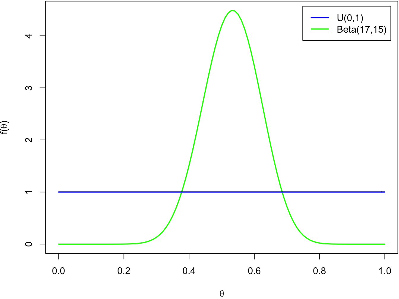
While the density of the prior distribution is flat, the density of posterior distribution is clearly concentrated near the value \(\theta = 0.5\). Now that have the full posterior distribution, we can easily compute the probabilities we were interested in:
1 - pbeta(0.5, alpha, beta) # P(theta > 0.5)## [1] 0.6399499pbeta(0.6, alpha, beta) - pbeta(0.4, alpha, beta) # P(0.4 < theta < 0.6)## [1] 0.7128906From the picture we can observe that almost all of the probability mass of the posterior distribution is between 0.2 and 0.8. Indeed, it is very likely that the true probability of the thumbtack landing point up really resides on this interval:
pbeta(0.8, alpha, beta) - pbeta(0.2, alpha, beta) # P(0.2 < theta < 0.8)## [1] 0.9996158We can also summarize the posterior distributions with a point estimate. In Bayesian statistics posterior mean, which is the mean of the posterior distribution is a widely used point estimate because of its optimality in the sense of mean squared error. A posterior mean in our thumbtacking example is a mean of the beta distribution: \[ E(\Theta|Y = y) = \frac{\alpha}{\alpha + \beta} = \frac{y+1}{(n-y+1) + (y + 1)} = \frac{y + 1}{n + 2}= \frac{17}{32}. \] This very close to the maximum likelihood estimate of this model, but both the numbers of failures and successes are inflated by one “pseudo-observation”. We will examine this phenomenon more closely in the next week when we discuss the choice of prior distributions.
1.2 Components of Bayesian inference
Let’s briefly recap and define more rigorously the main concepts of the Bayesian belief updating process, which we just demonstrated.
Consider a slightly more general situation than our thumbtack tossing example: we have observed a data set \(\mathbf{y} = (y_1, \dots, y_n)\) of \(n\) observations, and we want to examine the mechanism which has generated these observations. To this end, we model the observed data set as an observed value of the random vector \(\mathbf{Y} = (Y_1, \dots, Y_n)\).
In this course we limit ourselves to the parametric inference. Parametric inference is a special case of the statistical inference where it is assumed that the functional form of the joint distribution of the random vector \(\mathbf{Y}\) is fixed up to the value of the parameter vector \(\theta = (\theta_1, \dots, \theta_d) \in \Omega\) living in some parameter space \(\Omega\). The distribution of the data is written as the conditional distribution of the data given the parameter (because, as we remember, in Bayesian inference the parameter is considered as a random variable): \(f_{\mathbf{Y}|\Theta}(\mathbf{y}|\theta)\). This means that inference about the distribution of the data is reduced to finding out the distribution of the unknown parameter \(\Theta\). This simplifies the inference process significantly, because we can limit ourselves to the vector spaces instead of the function spaces.
Sampling distribution / likelihood function
Conditional distribution of the data set given the parameter, \(f_{\mathbf{Y}|\Theta}(\mathbf{y}|\theta)\), is called a sampling distribution, or the often simply a likelihood function.
More rigorously the sampling distribution means \(f_{\mathbf{Y}|\Theta}(\mathbf{y}|\theta)\) as a function of the observed data: \[ y \mapsto f_{\mathbf{Y}|\Theta}(\mathbf{y}|\theta), \] and likelihood function as a function of the parameter: \[ \theta \mapsto f_{\mathbf{Y}|\Theta}(\mathbf{y}|\theta), \] but often these terms are used interchangeably in practice (and also on this course).
Because our data set is a vector, in the general case a structure of the sampling distribution can be quite complicated. However, if we assume that our observations are independent (given the value of the parameter \(\Theta\)), denoted as \[ Y_1, \dots , Y_n \perp\!\!\!\perp | \Theta, \] the joint sampling distribution of random vector \(\mathbf{Y}\) can be factorized into a product of the sampling distributions of its components: \[ f_{\mathbf{Y}|\Theta}(\mathbf{y}|\theta) = \prod_{i=1}^n f_{Y_i|\Theta}(y_i|\theta). \] The situation is further simplified if our observations follow a same distribution. This situation is encountered quite often in this course, at least in the simplest examples. We say that random variables are independent and identically distributed (i.i.d.). In this case each of \(n\) components of the random vector \(\mathbf{Y}\) has a common sampling distribution \(f(y| \theta)\), and the joint sampling distribution can be further simplified to \[ f_{\mathbf{Y}|\Theta}(\mathbf{y}|\theta) = \prod_{i=1}^n f(y_i|\theta). \] In some cases, such as in our thumbtack tossing example the form of the sampling distribution (binomial distribution in this case) follows quite naturally from the structure of the expermintal situation. Other distributions that often follow naturally from the symmetry arguments or physical aspects of the examined phenomenon are multinomial distribution (extension of binomial experiment into the experiments with more than two possible outcomes, such as throwing a dice), normal distribution (sums or means of the independent random variables), Poisson distribution (occurrences of the independent events) and exponential distribution (waiting times or lifespans). In the more complex situations we cannot usually use any of these simple models directly, but we can try to build so called hierarchical models out of these basic distributions. Ultimately the choice of the sampling distribution is subjective, and up to our domain knowledge of the modelled phenomenon / and or computational convenience.
Prior distribution
A marginal distribution \(f_\Theta(\theta)\) of the parameter is called a prior distribution. Priori is latin for before: the prior distribution describes our beliefs about the likely values of the parameter \(\Theta\) before observing any data.
If we do not have any strong beliefs about the possible values of the parameter or we do not want let our beliefs to influence our results, we should choose as a vague priori distribution as possible, such as the uniform distribution in our thumbtack tossing example. This kind of the priori distribution is called an uninformative prior. But what we mean by “vague” here? It turns out that it is not possible to find a prior distribution that would be universally uninformative. For example uniform priors lead quickly to problems, if the parameter space is not restriced: how can you even define an uniform distribution over an interval of infinite length?
On the other hand, when we want to let our prior knowledge influence our posterior distribution, we set a stronger prior distribution. This kind of the prior distribution is called an informative prior. Informative prior distribution may be for example used to enforce sparsity into the model; this means we have a strong prior belief that some parameters of the model should be zero.
We will soon revisit uninformative and informative priors with a simple example.
The prior distribution for the parameter vector \(\Theta\) is also a parametric distribution; its parameters \(\phi = (\phi_1, \dots, \phi_k)\) are called hyperparameters. We can denote prior distribution also as \(f_{\Theta|\Phi}(\theta|\phi)\), but often the notation is simplified by leaving out the hyperparameters.
Bayesian model
To specify the fully Bayesian probability model, besides of the sampling distribution, we also need to specify the prior distribution of the parameter.
Together they determine the joint distribution of the observed data and the parameter: \[ f_{\Theta, \mathbf{Y}}(\theta, y) = f_\Theta(\theta)f_{\mathbf{Y}|\Theta}(\mathbf{y}|\theta). \] This full joint distribution is rarely computed or handled explicitly. Instead, the Bayesian inference is based on computing conditional and marginal densities from it.
Posterior distribution
The conditional distribution of the parameter given the data is called a posterior distribution. Posteriori is latin for after: posterior distribution describes our beliefs about the probable values of the parameter after we have observed the data.
In principle, the posterior distribution is computed from the prior and the sampling distributions using the Bayes’ theorem: \[ f_{\Theta|\mathbf{Y}}(\theta|\mathbf{y}) = \frac{f_{\Theta, \mathbf{Y}}(\theta, y)}{f_\mathbf{Y}(\mathbf{y})} = \frac{f_\Theta(\theta) f_{\mathbf{Y}|\Theta}(\mathbf{y}|\theta)}{f_\mathbf{Y}(\mathbf{y})}. \] In practice, we usually utilize the fact that the normalizing constant \(f_\mathbf{Y}(\mathbf{y})\) contains no \(\theta\); thus, it is a constant w.r.t. parameter \(\theta\). This means that we can compute the unnormalized density of the posterior distribution simply as a product of the sampling and prior distributions: \[ f_{\Theta|\mathbf{Y}}(\theta|\mathbf{y}) \propto f_\Theta(\theta) f_{\mathbf{Y}|\Theta}(\mathbf{y}|\theta), \] and then deduce the missing normalizing constant. In the first examples of this course this often done by recognizing the functional form of the familiar probability density.
Marginal likelihood
The normalizing constant \(f_\mathbf{Y}(\mathbf{y})\) of the Bayes’ theorem is called a marginal likelihood (sometimes also an evidence). It is computed by marginalizing out the parameter from the full joint probability distribution. For the continuous parameter this is done by integrating the joint probability distribution over the parameter space: \[ f_\mathbf{Y}(\mathbf{y}) = \int_\Omega f_\Theta(\theta)f_{\mathbf{Y}|\Theta}(\mathbf{y}|\theta) \,\text{d}\theta, \] and for the discrete parameter by summing the joint probability distribution over the parameter space: \[ f_\mathbf{Y}(\mathbf{y}) = \sum_{\theta \in \Omega} f_\Theta(\theta)f_{\mathbf{Y}|\Theta}(\mathbf{y}|\theta). \] If this averaging over all the possible parameter values seems a strange idea, it is probably easier to understand it by first considering the discrete case. You can for example take a look at the how the denominator of the Bayes’ theorem is computed in the classical drug testing example: Bayes’ theorem - Wikipedia.
In Bayesian data analysis (Gelman et al. 2013) the marginal likelihood is called a prior predictive distribution. This is because it presents our beliefs about the probabilities of the data before any observations are made. It is a distribution of the data computed as a weighted average over all the possible parameter values, and the weights are determined by the prior distribution.
If we denote \[ g(\mathbf{y}, \theta) := f_{\mathbf{Y}|\Theta}(\mathbf{y}|\theta), \] we can write the marginal likelihood as: \[\begin{equation} f_\mathbf{Y}(\mathbf{y}) = \int_\Omega g(\mathbf{y}, \theta) f_\Theta(\theta) \,\text{d}\theta =E[g(\mathbf{y},\Theta)], \tag{1.2} \end{equation}\]So the marginal likelihood can be written as an expectation of the sampling distribution, where the expectation is taken over the prior distribution of the parameter \(\Theta\)! Again, it may be easier to consider first a case of a discrete parameter, where the expectation is actually computed as an weighted average.
1.3 Prediction
1.3.1 Motivating example, part II
Let’s revisit the thumbtack tossing example: assume we have tossed a thumbtack \(n=30\) times, and observed that it has landed point up \(y=16\) times. But oftentimes instead of making inference about the parameters of the model, we are actually more interested in predicting the new observations. So what is our predictive distribution for the number of successes, if we throw the same thumbtack \(m=10\) more times?
Because the thumbtack stays the same, it makes sense to model the new throws as a sample from the same binomial distribution with the same successes probability as the original observations: \[ \tilde{Y} \sim \text{Bin}(m, \Theta) \] Further, it makes sense to model the old and the new observations independent given the parameter: \[ \tilde{Y},Y \perp\!\!\!\perp | \Theta. \] A naive way to obtain a probability mass function of \(\tilde{Y}\) would be just to plug the point estimate, such as a maximum likelihood estimate \(\hat{\theta}_{\text{MLE}}(y)\), as the parameter value of the probability mass function of the new observations: \(f_{\tilde{Y}|\Theta}(\tilde{y}|\hat{\theta}_{\text{MLE}}(y))\). However, by identifying the success probability the observed proportion of the successes, we run into the same problems as in the case of the parameter estimation: what if we had again observed a data \(y=0\) with \(n=3\)? Then the predictive distribution would assing a probability 1 to the value \(\tilde{Y} = n\), and probability 0 to all the other values. Surely we would have not needed any statistics to arrive at the conclusion that the thumbtack will land point down every time!
Instead, we will derive the proper Bayesian predictive distribution by actually computing the probability of the new observations given the observed data! This is denoted by \(f_{\tilde{Y}|Y}(\tilde{y}|y)\). We can immediately observe that the parameter theta does not exist at all in this formula. However, to derive the predictive distribution, we include the parameter as an auxiliary variable that is then integrated out. We first specify the joint distribution of the new observation \(\tilde{y}\) and the parameter \(\theta\) given the observed data \(\tilde{y}\), and then get the predictive distribution by integrating over the parameter space: \[\begin{equation} \begin{split} f_{\tilde{Y}|Y}(\tilde{y}|y) &= \int_\Omega f_{\tilde{Y}, \Theta|Y}(\tilde{y}|y) \,\text{d} \theta \\ &= \int_\Omega f_{\tilde{Y}|\Theta, Y}(\tilde{y}| \theta, y) f_{\Theta | Y}(\theta | y)\,\text{d} \theta \\ &= \int_\Omega f_{\tilde{Y}|\Theta}(\tilde{y}| \theta) f_{\Theta | Y}(\theta | y)\,\text{d} \theta. \end{split} \tag{1.3} \end{equation}\]In the second equality we used a chain rule for the conditional probabily densities: \[ f_{X,Y|Z} = f_{X|Y,Z} \,f_{Y|Z}, \] and in the final equality used a fact that the new observations are independent of the observed data given the parameter to simplify the expression. This predictive distribution \(f_{\tilde{Y}|Y}(\tilde{y}|y)\) of the new observations given the data we just derived is known as a posterior predictive distribution.
Now that we derived a general form of the posterior predictive distribution, we can plug the sampling distribution of the new observations \(f_{\tilde{Y}|\Theta}(\tilde{y}| \theta)\) and the posterior distribution \(f_{\Theta | Y}(\theta | y)\) we derived in the part one of this example, into this formula: \[ \begin{split} f_{\tilde{Y}|Y}(\tilde{y}|y) &= \int_\Omega f_{\tilde{Y}|\Theta}(\tilde{y}| \theta) f_{\Theta | Y}(\theta | y)\,\text{d} \theta \\ &= \int_0^1 \binom{m}{\tilde{y}} \theta^{\tilde{y}}(1-\theta)^{m-\tilde{y}} \frac{1}{B(\alpha_1, \beta_1)} \theta^{\alpha_1 - 1} (1- \theta)^{\beta_1 - 1} \,\text{d} \theta \\ &= \binom{m}{\tilde{y}} \frac{1}{B(\alpha_1, \beta_1)} \int_0^1 \theta^{\tilde{y} + \alpha_1 - 1}(1-\theta)^{m + \beta_1 -\tilde{y} - 1} \,\text{d} \theta. \end{split} \] To simplify the notation, we have denoted the parameters of the posterior distribution as \(\alpha_1 = y + 1\), and \(\beta_1 = n - y + 1\).
Next we are going to integrate in “a statistician way”: this means that we are not going to really integrate the expression, but we get rid of it by recognizing it as the integral whose value we know. We can do this by using one of the following tricks:
1. Explicitly recognize a familiar integral : We can immediately observe that the integral is a beta function (see eq. (1.1)), so we can write it more concisely as: \[ \int_0^1 \theta^{\tilde{y} + \alpha_1 - 1}(1-\theta)^{m + \beta_1 -\tilde{y} - 1} \,\text{d} \theta = B(\tilde{y} + \alpha_1, m + \beta_1 - \tilde{y}). \] 2. Recognize an unnormalized probability density function of the familiar distribution : We can also immediately observe that the integrand is a probability density function of the beta distribution Beta\((\tilde{y} + \alpha_1, m + \beta_1 - \tilde{y})\) up to a normalizing constant, and it is integrated over the support of the distribution. This means that if we add the missing normalizing constant, the integral is an integral of the probability density over its support: \[ \begin{split} &\int_0^1 \theta^{\tilde{y} + \alpha_1 - 1}(1-\theta)^{m + \beta_1 -\tilde{y} - 1} \,\text{d} \theta \\ = &B(\tilde{y} + \alpha_1, m + \beta_1 - \tilde{y}) \int_0^1 \frac{1}{B(\tilde{y} + \alpha_1, m + \beta_1 - \tilde{y})} \theta^{\tilde{y} + \alpha_1 - 1}(1-\theta)^{m + \beta_1 -\tilde{y} - 1} \,\text{d} \theta \\ &= B(\tilde{y} + \alpha_1, m + \beta_1 - \tilde{y}) \cdot 1 \\ &= B(\tilde{y} + \alpha_1, m + \beta_1 - \tilde{y}). \end{split} \] In this case the first trick was more straight-forward, but I also introduced the second one because in some cases recognizing the familiar integral requires performing a change of variables, and an unnormalized density function of the familiar distribution may be easier to recognize.
Whichever of these tricks you use, the posterior predictive distribution is simplified to \[ f_{\tilde{Y}|Y}(\tilde{y}|y) = \binom{m}{\tilde{y}} \frac{B(\tilde{y} + \alpha_1, m + \beta_1 - \tilde{y})}{B(\alpha_1, \beta_1)}. \] This a is probability distribution of the so called beta-binomial distribution, so we can denote our posterior predictive distribution as \[ \tilde{Y}|Y \sim \text{Beta-bin}(m, \alpha_1, \beta_1), \] where \(\alpha_1 = y + 1\), and \(\beta_1 = n - y + 1\) are the parameters of the posterior distribution for the parameter \(\Theta\).
1.3.2 Posterior predictive distribution
Let’s consider a general case: assume we have observations \(\mathbf{Y} = (Y_1, \dots , Y_n)\) with a sampling distribution \(f_{\mathbf{Y}|\Theta(\mathbf{y}|\theta)}\) conditional on the unknown parameter vector \(\Theta \in \Omega\). Now we want to predict the distribution for the \(m\) new observations \(\mathbf{\tilde{Y}} = (\tilde{Y}_1, \dots, \tilde{Y}_m)\) from the same process. Distribution \[
f_{\mathbf{\tilde{Y}} | \mathbf{Y}}(\mathbf{\tilde{y}}| \mathbf{y})
\] of the new observations given the observed data is called a posterior predictive distribution. If we further make a simplifying assumption that the new observations are independent of the observed data given the parameter, written as: \[
\mathbf{\tilde{Y}}, \mathbf{Y}\,|\, \Theta,
\] we can write the posterior predictive distribution as an integral \[
f_{\mathbf{\tilde{Y}} | \mathbf{Y}}(\mathbf{y}| \mathbf{y})
= \int_\Omega f_{\mathbf{\tilde{Y}}| \Theta}(\mathbf{\tilde{y}}| \theta) f_{\Theta|\mathbf{Y}}(\theta|\mathbf{y})\,\text{d}\theta,
\] which we derived in Equation (1.3). This formula may seem a little bit intimidating at first, but let’s try to find the intuition behind it. 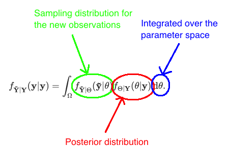 The integrand in the formula is a product of the sampling distribution for the new observations given the parameter, and the posterior distribution of the parameter given the old observations. When we denote the sampling distribution for the new observations as \[
g(\mathbf{\tilde{y}}, \theta) := f_{\mathbf{\tilde{Y}}| \Theta}(\mathbf{\tilde{y}}| \theta),
\] we can write the posterior predictive distribution as \[
f_{\mathbf{\tilde{Y}} | \mathbf{Y}}(\mathbf{y}| \mathbf{y})
= \int_\Omega g(\mathbf{\tilde{y}}, \theta) f_{\Theta|\mathbf{Y}}(\theta|\mathbf{y})\,\text{d}\theta
= E[g(\mathbf{\tilde{y}}, \theta) \,|\, \mathbf{Y = y}].
\] where the expectation is taken over the posterior distribution \(f_{\mathbf{Y}|\Theta}\). Like marginal likelihood (see Equation (1.2)), posterior predictive distribution is also a weighted average of the sampling distribution over the parameter values. However, the marginal likelihood was an unconditional expectation and the weights of the parameter values came from the prior distribution, whereas the posterior predictive distribution is a conditional expectation (conditioned on the observed data \(\mathbf{Y} = \mathbf{y}\)) and weights for the parameter values come from the posterior distribution.
The integrand in the formula is a product of the sampling distribution for the new observations given the parameter, and the posterior distribution of the parameter given the old observations. When we denote the sampling distribution for the new observations as \[
g(\mathbf{\tilde{y}}, \theta) := f_{\mathbf{\tilde{Y}}| \Theta}(\mathbf{\tilde{y}}| \theta),
\] we can write the posterior predictive distribution as \[
f_{\mathbf{\tilde{Y}} | \mathbf{Y}}(\mathbf{y}| \mathbf{y})
= \int_\Omega g(\mathbf{\tilde{y}}, \theta) f_{\Theta|\mathbf{Y}}(\theta|\mathbf{y})\,\text{d}\theta
= E[g(\mathbf{\tilde{y}}, \theta) \,|\, \mathbf{Y = y}].
\] where the expectation is taken over the posterior distribution \(f_{\mathbf{Y}|\Theta}\). Like marginal likelihood (see Equation (1.2)), posterior predictive distribution is also a weighted average of the sampling distribution over the parameter values. However, the marginal likelihood was an unconditional expectation and the weights of the parameter values came from the prior distribution, whereas the posterior predictive distribution is a conditional expectation (conditioned on the observed data \(\mathbf{Y} = \mathbf{y}\)) and weights for the parameter values come from the posterior distribution.
The posterior predictive distribution takes into account also the uncertainty of our parameter estimates, which is quantified by the posterior distribution. Thus, the variance of the posterior predictive distribution is in general higher than the variance of the sampling distribution into which a point estimate for the parameter \(\theta\), for example the maximum likelihood estimate or the posterior mean, is plugged.
1.3.3 Short note about the notation
In this introduction chapter we used quite a verbose notation: we explicitly wrote the random variables whose density functions we were handling as subscripts: for example we denoted the conditional density of random variable \(\mathbf{Y}\) given \(\Theta = \theta\) as: \[ f_{\mathbf{Y}|\Theta}(\mathbf{y}|\theta). \] This makes it immediately clear which densities we are handling, but when the formulas get longer, using this heavy notation may become quite cumbersome. This is why in statistics and machine learning literature a more concise notation is generally used. In this slight abuse of notation all the density and probability mass functions are denoted with the same letter (usually \(p\)) without any subscripts. The random variables whose density functions they are can be recognized by the arguments of the densities. For example the conditional density \(f_{\mathbf{Y}|\Theta}(\mathbf{y}|\theta)\) is written concisely as \(p(\mathbf{y}|\theta)\), and the Bayes’ theorem can be written as \[ p(\theta|\mathbf{y}) = \frac{p(\theta) p(\mathbf{y}|\theta)}{p(\mathbf{y})}. \] This shorthand notation makes formulas shorter and more clear to read assuming that you know in the first place for which it is shorthand for. In the following chapters we will use this notation.
Often also the random variables and their realizations are denoted with the same lowercase letter if there is no risk of confusion. This is particularly the case with the parameters, in part because there exist no useful uppercase versions of many greek alphabets. So when we talk about “the parameter \(\theta\)” in the following chapters, you have to remember that usually a random variable is meant.
References
Gelman, A., J.B. Carlin, H.S. Stern, D.B. Dunson, A. Vehtari, and D.B. Rubin. 2013. Bayesian Data Analysis, Third Edition. Chapman & Hall/Crc Texts in Statistical Science. Taylor & Francis. https://books.google.fi/books?id=ZXL6AQAAQBAJ.