Chapter 2 Conjugate distributions
Conjugate distribution or conjugate pair means a pair of a sampling distribution and a prior distribution for which the resulting posterior distribution belongs into the same parametric family of distributions than the prior distribution. We also say that the prior distribution is a conjugate prior for this sampling distribution.
A parametric family of distributions \[ \{f_{Y|\Theta}(y|\theta) : \theta \in \Omega \} \] means simply a set of distributions which have a same functional form, and differ only by the value of the finite-dimensional parameter \(\theta \in \Omega\). For instance, all beta distributions or all normal distributions form a parametric families of distributions.
We have already seen one example of the conjugate pair in the thumbtack tossing example: the binomial and the beta distribution. You may now be wondering: “But Ville, in our example the prior distribution was an uniform distribution, not a beta distribution??” It turns out that the prior was indeed a beta distribution, because the uniform distribution U\((0,1)\) is actually a same distribution than the beta distribution Beta\((1,1)\) (check that this holds!).
Using conjugate pairs of distributions makes a life of the statistician more convenient, because the marginal likelihood, and thus also the posterior distribution and the posterior predictive distribution can be solved in a closed form. Actually, it turns out that this is the second of the only two special cases in which this is possible:
- The parameter space is discrete and finite: \(\Omega = (\theta_1, \dots, \theta_p)\); in this case the marginal likelihood can be computed as a finite sum: \[ f_{Y}(\mathbf{y}) = \sum_{i=1}^p f_{\mathbf{Y}|\Theta}(\mathbf{y_i}|\theta_i) f_{\Theta}(\theta_i). \]
- The prior distribution is a conjugate prior for the sampling distribution.
In all the other cases we have to approximate the posterior distributions and the posterior predictive distributions. Usually this is done by simulating values from them; we will return to this topic soon.
2.1 One-parameter conjugate models
When parameter \(\Theta \in \Omega\) is a scalar, the inference is particularly simple. We have already seen one example of the one-parameter conjugate model (the thumbtacking example), but let’s examine another simple model.
2.1.1 Example: Poisson-gamma model
A Poisson distribution is a discrete distribution which can get any non-negative integer values. It is a natural distribution for modelling counts, such as goals in a football game, or a number of bicycles passing a certain point of the road in one day. Both the expected value and the variance of a Poisson distributed random variable are equal to the parameter of the distribution: if \(Y \sim\) Poisson\((\lambda)\), \[ E[Y] = \lambda, \quad Var[Y] = \lambda. \]
Let’s cheat a little bit this time: we will first generate observations from the distribution with a known parameter, and then try estimate the posterior distribution of the parameter from this data:
n <- 5
lambda_true <- 3

# set seed for the random number generator, so that we get replicable results
set.seed(111111)
y <- rpois(n, lambda_true)
y
## [1] 4 3 11 3 6Now we actually know that the true generating distribution of our observations \(y=(4, 3, 11, 3 , 6)\) is Poisson(3); but lets forget this for a moment, and proceed with the inference.
Assume that the observed variables are counts, which means that they can in principle take any non-negative integer value. Thus, it is natural to model them as independent Poisson-distributed random variables: \[ Y_1, \dots, Y_n \sim \text{Poisson}(\lambda) \perp\!\!\!\perp \,|\, \lambda \]
Because the parameter of the Poisson distribution can in principle be any positive real number, we want use a prior whose support is \((0, \infty)\). If we used for example an uniform prior \(U(0,100)\), posterior density would also be zero outside of this interval, even if all the observations were greater than 100. So usually we want a prior that assings a non-zero density for all the possible parameter values.
It is not possible to set a uniform distribution over the infinite interval \((0,\infty)\), so we have to come up with something else. A gamma distribution is a convenient choice. It is a distribution with a peak close to zero, and a tail that goes to infinity. It also turns out that the gamma distribution is a conjugate prior for the Poisson distribution: this means tha we can actually solve the posterior distribution in a closed form.
We can set the parameters of the prior distribution for example to \(\alpha = 1\) and \(\beta = 1\); we will examine the choice of both the prior distribution and its parameters (called hyperparameters) later. For now on, let’s just solve the posterior with the conjugate gamma prior: \[ \lambda \sim \text{Gamma}(\alpha, \beta). \] Because the observations are independent given the parameter, a likelihood function for all the observations \(\mathbf{Y} = (Y_1, \dots, Y_n)\) can be written as a product of the Poisson distributions: \[ p(\mathbf{y}|\lambda) = \prod_{i=1}^n p(y_i|\lambda) = \prod_{i=1}^n \lambda^{y_i} \frac{e^{-\lambda}}{y_i!} \propto \lambda^{\sum_{i=1}^n y_i} e^{-n\lambda} = \lambda^{n\overline{y}} e^{-n\lambda}, \] where \[ \overline{y} = \frac{1}{n} \sum_{i=1}^n y_i \] is a mean of the observations. Again we dropped the constant terms which do not depend on the parameter from the expression of the likelihood.
The unnormalized posterior distribution for the parameter \(\lambda\) can now be written as \[\begin{equation} \begin{split} p(\lambda|\mathbf{y}) &\propto p(\mathbf{y}|\lambda)p(\lambda) \\ &\propto \lambda^{n\overline{y}} e^{-n\lambda}\lambda^{\alpha-1} e^{-\beta\lambda} \\ &= \lambda^{\alpha + n\overline{y} - 1} e^{-(\beta + n) \lambda}. \end{split} \tag{2.1} \end{equation}\]The gamma prior was chosen because a gamma distribution is a conjugate prior for the Poisson distribution, and indeed we can recognize the unnormalized posterior distribution as the kernel of the gamma distribution. Thus, the posterior distribution is \[ \lambda \,|\, \mathbf{Y} \sim \text{Gamma}(\alpha + n\overline{y}, \beta + n). \]
We can now plot the prior and the posterior distributions:
alpha <- 1
beta <- 1

lambda <- seq(0,7, by = 0.01) # set up grid for plotting
plot(lambda, dgamma(lambda, alpha, beta), type = 'l', lwd = 2, col = 'orange',
     ylim = c(0, 3.2), xlab = expression(lambda),
     ylab = expression(paste('p(', lambda, '|y)')))
lines(lambda, dgamma(lambda, alpha + sum(y), beta + n),
      type = 'l', lwd = 2, col = 'violet')
abline(v = lambda_true, lty = 2)
legend('topright', inset = .02, legend = c('prior', 'posterior'),
       col = c('orange', 'violet'), lwd = 2)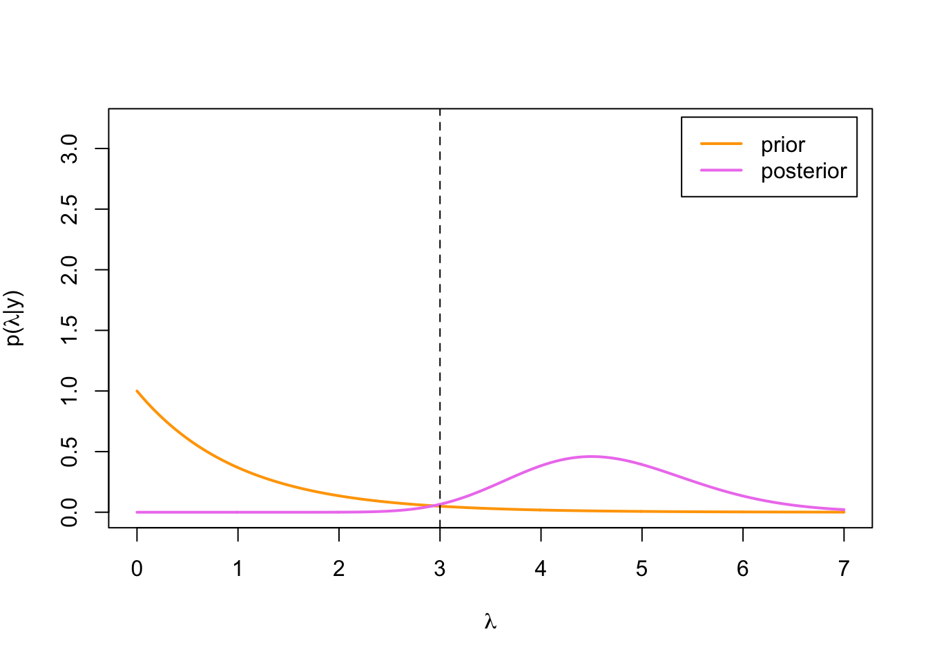
We can see that the posterior distribution is concentrated quite a bit higher than the true parameter value. This is because our third observation happened to be a bit of an outlier: the probability of drawing a value of 11 or higher from Poisson(3)-distribution (if we draw only one value), is only:
ppois(10,3, lower.tail = FALSE)## [1] 0.000292337But because we are anyway using simulated data, let’s draw some more observations from the same Poisson(3)-distribution:
n_total <- 200
set.seed(111111) # use same seed, so first 5 obs. stay same
y_vec <- rpois(n_total, lambda_true)
head(y_vec)
## [1] 4 3 11 3 6 3and plot the posterior distributions with different sample sizes to see if things even out:
n_vec <- c(1, 2, 5, 10, 50, 100, 200)

par(mfrow = c(4,2), mar = c(2, 2, .1, .1))

plot(lambda, dgamma(lambda, alpha, beta), type = 'l', lwd = 2, col = 'orange',
     ylim = c(0, 3.2), xlab = '', ylab = '')
abline(v = lambda_true, lty = 2)
text(x = 0.5, y = 2.5, 'prior', cex = 1.75)

for(n_crnt in n_vec) {
  y_sum <- sum(y_vec[1:n_crnt])
  plot(lambda, dgamma(lambda, alpha, beta), type = 'l', lwd = 2, col = 'orange',
       ylim = c(0, 3.2), xlab = '', ylab = '')
  lines(lambda, dgamma(lambda, alpha + y_sum, beta + n_crnt),
        type = 'l', lwd = 2, col = 'violet')
  abline(v = lambda_true, lty = 2)
  text(x = 0.5, y = 2.5, paste0('n=', n_crnt), cex = 1.75)
}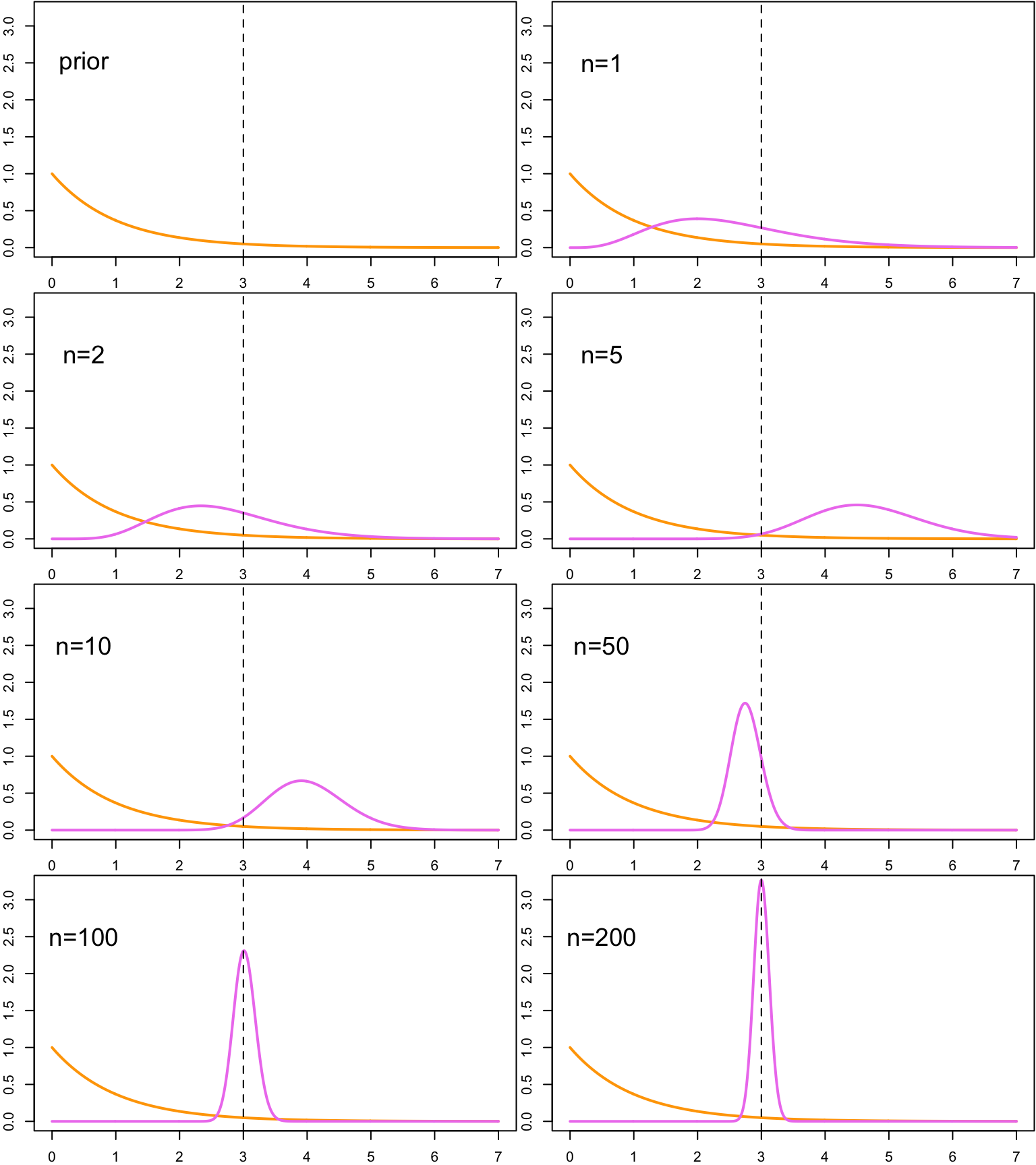
After the first two observations the posterior is still quite close to the prior distribution, but the third observation, which was an outlier, shifts the peak of the posterior from the left side of the mean heavily to the right. But when more observations are drawn, we can observe that the posterior starts to concentrate more heavily on the neighborhood of the true parameter value.
2.1.2 Example: prediction in Poisson-gamma model
Let’s denote the parameters of the posterior distribution computed in the previous example as \[ \alpha_1 := \alpha + n\overline{y} \] and \[ \beta_1 := \beta + n, \] and solve the posterior predictive distribution for one new observation \(\tilde{Y}_1\) from the same Poisson distribution as the observed data: \[ \tilde{Y}_1, Y_1, \dots , Y_n \sim \text{Poisson}(\lambda) \perp\!\!\!\perp \,|\, \lambda. \] The posterior predictive distribution for \(\tilde{Y}_1\) can be written as: \[ \begin{split} p(\tilde{y}_1 | \mathbf{y}) &= \int_\Omega p(\tilde{y}_1 | \lambda) p(\lambda|\mathbf{y}) \, \text{d}\lambda \\ &= \int_0^\infty \lambda^{\tilde{y}_1} \frac{e^{-\lambda}}{\tilde{y}_1!} \frac{\beta_1^{\alpha_1}}{\Gamma(\alpha_1)} \lambda^{\alpha_1 - 1} e^{-\beta_1\lambda} \,\text{d}\lambda \\ &= \frac{\beta_1^{\alpha_1}}{\Gamma(\alpha_1)\tilde{y}_1!} \int_0^\infty \lambda^{\tilde{y}_1 + \alpha_1 - 1} e^{-(\beta_1+1)\lambda} \, \text{d}\lambda. \end{split} \] Now it would be probably easiest to use the first of the tricks introduced in Example 1.3.1, and complete the integral into an integral of a gamma density over its support. But just to make things more interesting, let’s use the second trick by completing it into a gamma function by the following change of variables: \[ t = (\beta_1 + 1) \lambda. \] Now \[ \lambda = g(t) := \frac{t}{\beta_1 + 1}, \] and \[ \quad \text{d}\lambda = g'(t) \,\text{d}\text{t} = \frac{1}{\beta_1 + 1} \,\text{d}\text{t}. \] This change of variables is only a multiplication by a positive constant, so it has no effect on the limits of the integral. After performing the change of variables we can recognize the gamma integral: \[ \begin{split} \int_0^\infty \lambda^{\tilde{y}_1 + \alpha_1 - 1} e^{-(\beta_1+1)\lambda} \, \text{d}\lambda &= \int_0^\infty \left(\frac{t}{\beta_1 + 1}\right)^{\tilde{y}_1 + \alpha_1 - 1} e^{-t} \frac{1}{\beta_1 + 1} \, \text{d}t \\ &= \left(\frac{1}{\beta_1 + 1}\right)^{\tilde{y}_1 + \alpha_1} \int_0^\infty t^{\tilde{y}_1 + \alpha_1 - 1} e^{-t}\, \text{d}t \\ &= \left(\frac{1}{\beta_1 + 1}\right)^{\tilde{y}_1 + \alpha_1} \Gamma(\tilde{y}_1 + \alpha_1). \end{split} \] Thus, we can write the posterior predictive density as \[ \begin{split} p(\tilde{y}_1 | \mathbf{y}) &= \frac{\beta_1^{\alpha_1}}{\Gamma(\alpha_1)\tilde{y}_1!} \cdot \left(\frac{1}{\beta_1 + 1}\right)^{\tilde{y}_1 + \alpha_1} \Gamma(\tilde{y}_1 + \alpha_1) \\ &= \frac{\Gamma(\tilde{y}_1 + \alpha_1)}{\Gamma(\alpha_1)\tilde{y}_1!} \left(\frac{1}{\beta_1 + 1}\right)^{\tilde{y}_1} \left(\frac{\beta_1}{\beta_1 + 1}\right)^{\alpha_1} \\ &=\frac{\Gamma(\tilde{y}_1 + \alpha_1)}{\Gamma(\alpha_1)\tilde{y}_1!} \left(1 - \frac{\beta_1}{\beta_1 + 1}\right)^{\tilde{y}_1} \left(\frac{\beta_1}{\beta_1 + 1}\right)^{\alpha_1}. \end{split} \] This is a density function of the following negative binomial distribution: \[ \tilde{Y}_1 \,|\, \mathbf{Y} \sim \ \text{Neg-Bin}\left(\alpha_1, \frac{\beta_1}{\beta_1 + 1}\right). \] Still assuming that our prior was Gamma\((1,1)\)-distribution, we can compare this posterior predictive distribution to the true generative distribution of the data:
y_grid <- 0:15
alpha_1 <- alpha + sum(y)
beta_1 <- beta + n

plot(y_grid, dnbinom(y_grid, size = alpha_1, prob = beta_1 / (1 + beta_1)),
     type = 'h', lwd = 3, col = 'violet', xlab = expression(tilde(y)),
     ylab = 'probability', ylim = c(0, 0.25))
lines(y_grid, dnbinom(y_grid, size = alpha_1, prob = beta_1 / (1 + beta_1)),
      type = 'p', lwd = 3, col = 'violet')
lines(y_grid, dpois(y_grid, lambda_true), type = 'b', lwd = 3, col = 'mediumseagreen')
legend('topright', inset = .02,
       legend = c('posterior predictive', 'true distribution'),
       col = c('violet', 'mediumseagreen'), lwd = 3)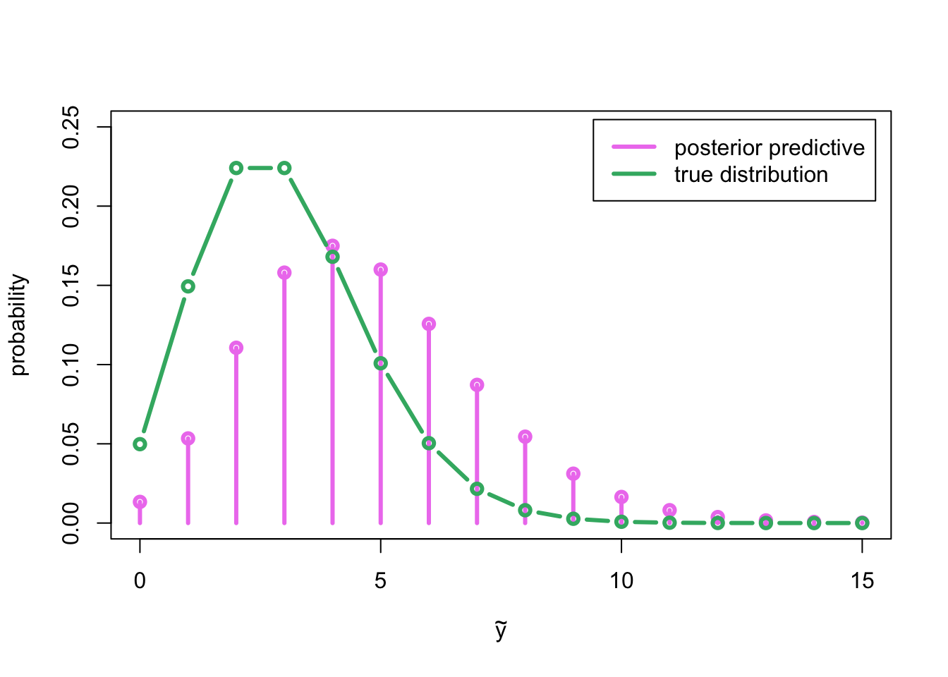
As could be expected based on the posterior distribution for parameter \(\lambda\), which was concentrated on the larger values than the true value \(\lambda = 3\), also the posterior predictive distribution is concentrated (remember that the expected value of Poisson distribution is its parameter) on the higher values compared to the generating distribution Poisson\((3)\).
Let’s see what the posterior predictive distribution looks like for the different sample sizes (using the data we generated earlier):
par(mfrow = c(4,2), mar = c(4, 4, .1, .1))

plot(y_grid, dnbinom(y_grid, size = alpha, prob = beta / (1 + beta)),
     type = 'h', lwd = 3, col = 'violet', xlab = expression(tilde(y)),
     ylab = 'probability', ylim = c(0, 0.5))
lines(y_grid, dnbinom(y_grid, size = alpha, prob = beta / (1 + beta)),
      type = 'p', lwd = 3, col = 'violet')
lines(y_grid, dpois(y_grid, lambda_true), type = 'b', lwd = 3, col = 'mediumseagreen')
text(x = 11, y = 0.4, 'marginal likelihood', cex = 1.75)

for(n_crnt in n_vec) {
  y_sum <- sum(y_vec[1:n_crnt])
  alpha_1 <- alpha + y_sum
  beta_1 <- beta + n_crnt
  plot(y_grid, dnbinom(y_grid, size = alpha_1, prob = beta_1 / (1 + beta_1)),
       type = 'h', lwd = 3, col = 'violet', xlab = expression(tilde(y)),
       ylab = 'probability', ylim = c(0, 0.5))
  lines(y_grid, dnbinom(y_grid, size = alpha_1, prob = beta_1 / (1 + beta_1)),
        type = 'p', lwd = 3, col = 'violet')
  lines(y_grid, dpois(y_grid, lambda_true), type = 'b', lwd = 3, col = 'mediumseagreen')
  text(x = 12, y = 0.4, paste0('n=', n_crnt), cex = 1.75)
}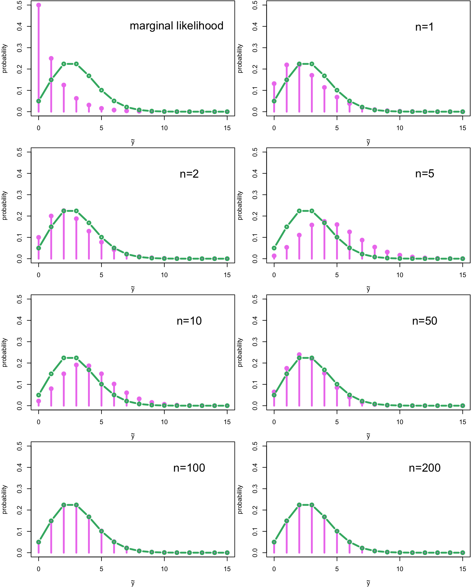
The first plot contains actually the marginal likelihood for one observation \(Y_1\): \[ p(y_1) = \int_\Omega p(y_1|\lambda)p(\lambda)\, \text{d} \lambda \] This marginal likelihood is Neg-bin\(\left(\alpha, \frac{\beta}{\beta + 1}\right)\)-distribution. We already basicly derived this when we computed the posterior predictive distribution; the only difference was in the parameters of the gamma distribution. This also holds in a more general case: the derivation for the marginal likelihood and the posterior predictive distribution is the same; the only difference is in the value of the parameters of the conjugate prior distribution. This means that every time we can solve the posterior distribution in a closed form, we can also solve the posterior predictive distribution!
But I digress… Let’s look at the plots again: when we have only one or two observations, the posterior predictive distribution is closer to the marginal likelihood. Again, the third observation, which was the outlier, tilts the posterior predictive distribution immediately towards the higher values, until the it starts to resemble more or less the true generating distribution when more data is generated.
This is recurring theme in a Bayesian inference: when the sample size is small, the prior has more influence on the posterior, but when the sample size grows, the data starts to influence our posterior distribution more and more, until at the limit the posterior is determined purely by the data (at least when the certain conditions hold). Examining the case \(n \rightarrow \infty\) is called asymptotics, and it is a cornerstone of the statistical inference, but we do not have time go very deep into this topic on this course.
Now you may be thinking: “But if have enough data, then we do not have to care about the priors, don’t we?” Well, in this case you are lucky, but before you can forget about the priors, you have to ask yourself (at least) two things:
How complex model you want to fit? In general, more complex the model, more data you need. For example modern deep learning models may have millions of parameters, so probably a sample size of \(n=50\) is not “high enough”, although this was the case in our toy example.
In what resolution level you want examine your data? You may have enough data to fit your model at the level of the country, but what if you want to model the differences between the towns? Or the neighborhoods? We will actually have a concrete example of this exact situation on the exercises later.
2.2 Prior distributions
The most often criticized aspect of the Bayesian approach to statistical inference is the requirement to choose a prior distribution, and especially the subjectivity of this prior selection procedure. The Bayesian answer to this criticism is to point out that the whole modeling procedure is inherently subjective: it is never possible for the data to fully “speak for itself” because we have to always make some assumptions about its sampling distribution.
Even in the most trivial coin-flipping example the choice of the binomial distribution for the outcome of the coinflip can be questioned: if we were truly ignorant about the outcome of the coinflip, would it make sense to model the outcome with a trinomial distribution, where the outcomes were head, tails and the coin landing on its side? So even the choice of the restricting the parameter space to \(\Omega = \{\text{heads}, \text{tails}\}\) is based on the our prior knowledge about the previous coinflips and the common sense knowledge that the coin landing on its side is almost impossible. It can be argumented that we always use somehow our prior knowledge in the modelling process, but the Bayesian framework just makes utilizing prior knowledge more transparent and easier to quantify.
A less philosophical and more practical example of the inherent subjectivity of the modelling process is any situation in which our observations are continuous instead of the discrete. For instance, let’s consider a classical statistical problem of estimating the true population distribution of some quantity, say the average height of adult females, on the basis of the subsample from some human population. Assume that we have measured the following heights of the five people from this population, say some tribe in South America (in metres): \[ \mathbf{y} = (1.563, 1.735, 1.642, 1.662, 1.528). \] Now we could of course “let the data speak for itself”, and assume that the true distribution of the height of the females of this tribe is the empirical distribution of our observations: \[ P(Y = y) = \begin{cases} 1/5 \quad &\text{if} \,\, y = 1.563, \\ 1/5 \quad &\text{if} \,\, y = 1.735, \\ 1/5 \quad &\text{if} \,\, y = 1.642, \\ 1/5 \quad &\text{if} \,\, y = 1.662, \\ 1/5 \quad &\text{if} \,\, y = 1.528, \\ 0 \quad &\text{otherwise}. \end{cases} \] But this would of course be an absurd conclusion. In practice, we have to impose some kind of the sampling distribution, for example the normal distribution, for the observations for our inferences to be sensible. Even if we do not want to impose any parametric distribution on the data, we have to choose some nonparameteric method to smooth a height distribution.
So this is the Bayesian counter-argument: the choice of the sampling distribution is as subjective as the choice of the prior distribution. Take for instance a classical linear regression. It makes huge simplifying assumptions: that the true that the error terms are normally distributed given the predictors, and that the parameters of this normal distribution do not depend on the values of the predictors. Also the choices of the predictors inject very strong subjective beliefs into the model: if we exclude some predictors from the model, this means that we assume that this predictor has no effect at all on the output variable. If we do not include any second or higher order terms, this means that we make a rather dire assumption that the all the relationships between the predictors and the output variables are linear, and so on.
Of course the models with different predictors and model structures can be tested (for example by predicting on the test set or by cross-validation), and then the best model can be chosen, but the same thing can be also done for the prior distributions. So we do not have to choose the first prior distribution or hyperparameters that we happen to test, but like the different sampling distributions, we can also test different prior distributions and hyperparameter values to see which of them make sense. This kind of the comparing the effects of the choice of prior distribution is called sensitivity analysis.
Besides being the most criticized aspect of the Bayesian inference, the choice of the prior distribution is also one of the hardest. Often there are not any ‘’righ’’ priors, but the usual choices are often based on the computational convenience or desired statistical properties.
2.2.1 Informative priors
If we have prior knowledge about the possible parameter values, it often makes sense to limit the sampling to these parameter values. The prior distribution which is designed to encode our prior knowledge of the likely parameter values and to affect the posterior distribution with small sample sizes is called an informative prior. Using informative prior often makes the solution more stable with the smaller sample sizes, and on the other hand the sampling from the posterior is often more efficient when informative prior is used, because then we do not waste too much energy sampling the highly improbable regions of the parameter space.
However, when using an informative prior distribution, it is better to use soft instead of the hard restrictions on the possible parameter values. Let’s illustrate this by returning to the problem of estimating the distribution of the mean height of the females of some population, and assume that we model the height by the normal distribution \(N(\mu, \sigma^2)\). Because the estimated parameter \(\mu\) is a mean of the height of adult females, it would make sense to limit the possible parameter values to the interval \((0.5,2.5)\) because clearly it is impossible for the mean height of the adults be outside of this interval; this can be done by using as a prior the uniform distribution \[ \mu \sim U(0.5, 2.5). \] This prior has the probability mass of zero outside of this interval; thus also the value of the posterior distribution for \(\mu\) is zero outside of this interval. In this example it actually makes sense to use this kind of the prior because it is based on the natural constraints of the human height. However, in general this approach has two weaknesses:
- If the posterior mean falls near one of the limits of this interval, the interval ‘’cuts’’ the posterior distribution. Also the sampling works worse near the limit.
- Often this kind of the uniform prior on the interval gives undue influences to the extreme values which are near the limits.
Both of these problems can be circumvented by using a prior which has most of its probability mass on the interval where the true parameter value is assumed to surely lie, but that does not limit it to this interval. For this example this kind of the prior which sets ‘’soft’’ limits to the parameter values would be for example the normal distribution with mean \(1.5\) and variance \(0.15\): \[ \mu \sim N(1.5, 0.15). \] This normal distribution has approximately \(99\%\) of its probability mass (pink area under the curve) on the interval \((0.5, 2.5)\), but does not limit the parameter values to this interval1:
x <- seq(0,3, by = .001)
mu <- 1.5
sigma <- sqrt(.15)
plot(x, dnorm(x, mu, sigma), type = 'l', col = 'red', lwd = 2, ylab = 'Density')

q_lower <- qnorm(.005, mu, sigma)
q_upper <- qnorm(.995, mu, sigma)
y_val <- dnorm(x, mu, sigma)
x_coord <- c(q_lower, x[x >= q_lower & x <= q_upper], q_upper)
y_coord <- c(0, y_val[x >= q_lower & x <= q_upper], 0)
polygon(x_coord, y_coord, col = 'pink', lwd = 2,  border = 'red')
legend('topright', legend='N(1.5, 0.15)', col='red', inset=.1, lwd=2, bty='n')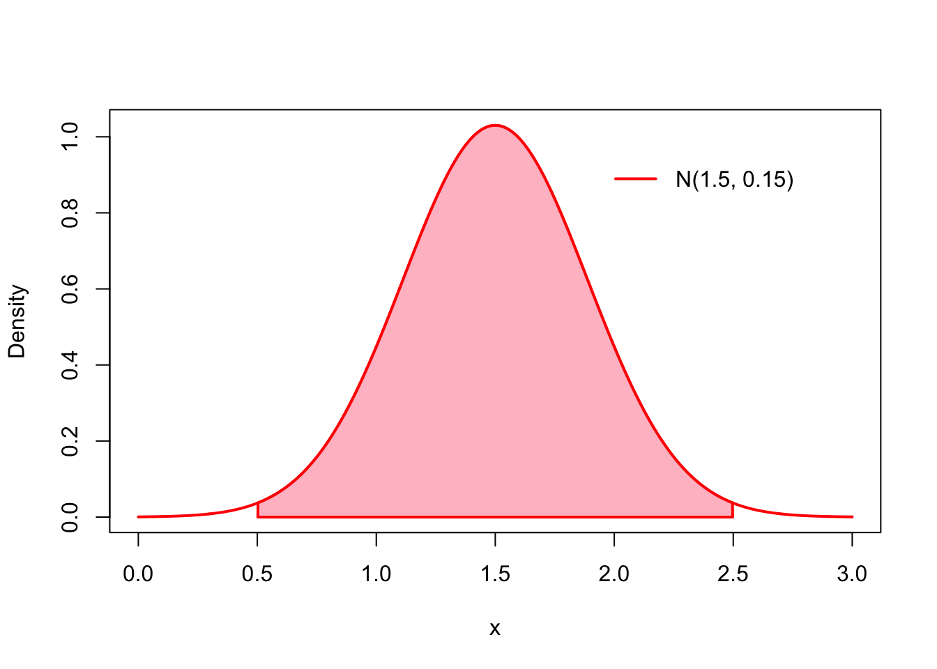
This distribution has also a pleasant property that it pulls the posterior distribution towards the center of the distribution. Informative priors can be based on our prior knowledge of the examined phenomenon. For instance, this prior distribution may be an observed distribution of the means of the heights of the females of the all South-American tribes measured. We will return to the topic of combining inferences from the several subpopulations in the chapter about hierarchical models. If there is no this kind of the prior knowledge, it is better to use a non-informative prior, or at least to set a variance of the prior quite high.
2.2.2 Non-informative priors
A non-informative or uninformative prior is a prior distribution which is designed to influence the posterior distribution as little as possible. It makes sense to use a non-informative prior in situations in which we do not have any clear prior beliefs about the possible parameter values, or we do not want these prior beliefs to influence the inference proces.
Non-informative and informative prior are not formally defined terms. They are better be thought as a continuum: some prior distributions are more informative than others. However, often some prior distribution are clearly non-informative and some are informative, but it is important to remember that this distinction is just a heuristic, not any definition.
But what kind of the prior distribution is non-informative? An intuitive answer would be an uniform distribution. This was also a suggestion of the pioneers of the Bayesian inference, Bayes and Laplace. But as we observed in the beta-binomial example 1.1.3, in the binomial model with beta prior the uniform prior \(\text{Beta}(1,1)\) actually corresponds to having two pseudo-observations: one failure and one success. So it is not completely uninformative. Another problem with the uniform priors are that they are not invariant with respect to parametrization: if we change to parametrization of the likelihood, the prior is not uniform anymore. We will explore this phenomenon for the beta-binomial model in the exercises.
2.2.3 Improper priors
Often the distributions are most non-informative near the limits of their parameter space. For instance, the parameters of the beta prior \(\text{Beta}(\alpha, \beta)\) can be thought as the (possibly non-integer) pseudo-observations: \(\alpha\) represents pseudo-successes, and \(\beta\) represents pseudo-failures. With this logic the most non-informative prior would be \(\text{Beta}(0,0)\). But the problem with this prior is that it is not a probability distribution, because the Beta function approaches infinity when the parameters \(\alpha, \beta \rightarrow 0\).
However, it turns out that we can plug this kind of the function that cannot be normalized into the proper probability distribution into the place of the prior in the Bayes’ theorem, as long the resulting posterior distribution is a proper probability distribution. We call this kind of the priors that are not densities of any probability distribution as improper priors.
In the beta-binomial example we can denote the aforementioned improper prior (known as Haldane’s prior) as: \[ p(\theta) \propto \theta^{-1}(1-\theta)^{-1}. \] It can be easily shown that the resulting posterior is proper a long as we have observes at least one success and one failure.
Improper priors are often obtained as the limits of the proper priors, and they are often used because they are non-informative. We can demonstrate both of these properties with our height estimation example: the noninformative prior for the average height \(mu\) would be an uniform distribution over the whole real axis: \[ p(\mu) \propto 1. \] But of course this cannot be normalized into the probability distribution by dividing it by its integral over the real axis, because this integral is infinite. However, the resulting posterior is a normal distribution if we have at least one observation (assuming known variance). This improper prior can also be interpreted as a normal distribution with infinite variance.
When using improper priors, it is important to check that the resulting posterior is a proper probability distribution.
Of course the height cannot be negative… maybe it could be better to choose a gamma or some other distribution whose support is positive real axis for our prior. But the normal distribution is a very convenient choice for this example because its parameters have direct interpretations as the mean and the variance of the distribution.↩