Chapter 6 Hierarchical models

Often observations have some kind of a natural hierarchy, so that the single observations can be modelled belonging into different groups, which can also be modeled as being members of the common supergroup, and so on. For instance, the results of the survey may be grouped at the country, county, town or even neighborhood level. This kind of the spatial hierarchy is the most concrete example of the hierarchy structure, but for example different clinical experiments on the effect of the same drug can be also modeled hierarchically: the results of each test subject belong to the one of the experiments (=groups), and these groups can be modeled as a sample from the common population distribution. This kind of the combining of results of the different studies on the same topic is called meta-analysis.

Often the observations inside one group can be modeled as independent: for instance, the results of the test subjects of the randomized experiments, or responses of the survey participant chosen by the random sampling can be reasonably thought to be independent. On the other hand, the parameters of the groups, for example mean response of the test subjects to the same drug in the different clinical experiments, can hardly be thought as independent. However, because the experimental conditions, for example the age or other attributes of the test subjects, length of the experiment and so on, are likely to affect the results, it also does not feel right to assume the are no differences at all between the groups by pooling all the observations together.

The idea of the hierarchical modeling is to use the data to model the strength of the dependency between the groups. The groups are assumed to be a sample from the underlying population distribution, and the variance of this population distribution, which is estimated from the data, determines how much the parameters of the sampling distribution are shrunk towards the common mean.

First we will take a look at the general form of the two-level hierarchical model, and then make the discussion more concrete by carefully examining a classical example of the hierarchical model.

6.1 Two-level hierarchical model

The most basic two-level hierarchical model, where we have \(J\) groups, and \(n_1, \dots n_J\) observations from each of the groups, can be written as \[ \begin{split} Y_{ij} \,|\, \boldsymbol{\theta}_j &\sim p(y_{ij} | \boldsymbol{\theta}_j) \quad \text{for all} \,\, i = 1, \dots , n_j \\ \boldsymbol{\theta}_j \,|\, \boldsymbol{\phi} &\sim p(\boldsymbol{\theta}_j | \boldsymbol{\phi}) \quad \text{for all} \,\, j = 1, \dots, J. \\ \end{split} \] for each of the \(j = 1, \dots, J\) groups.

We assume that the observations \(Y_{1j}, \dots , Y_{n_jj}\) within each group are i.i.d., so that the joint sampling distribution can be written as a product of the sampling distributions of the single observations (which were assumed to be the same): \[ p(\mathbf{y}_j |\boldsymbol{\theta}_j) = \prod_{i=1}^{n_j} p(y_{ij}|\boldsymbol{\theta}_j). \] Group-level parameters \((\boldsymbol{\theta}_1, \dots, \boldsymbol{\theta}_J)\) are then modeled as an i.i.d. sample from the common population distribution \(p(\boldsymbol{\theta}_j | \boldsymbol{\phi})\) so that their joint distribution can also be factorized as: \[ p(\boldsymbol{\theta}|\boldsymbol{\phi}) = \prod_{j=1}^J p(\boldsymbol{\theta}_j | \boldsymbol{\phi}). \] The full model specification depends on how we handle the hyperparameters. We will introduce three options:

1. fix them to some constant values,
2. use a point estimates estimated from the data or
3. set a probability distribution over them.

When we speak about the Bayesian hierarchical models, we usually mean the third option, which means specifying the fully Bayesian model by setting the prior also for the hyperparameters.

6.1.1 No-pooling model

If we just fix the hyperparameters to some fixed value \(\boldsymbol{\phi} = \boldsymbol{\phi}_0\), then the posterior distribution for the parameters \(\boldsymbol{\theta}\) simply factorizes to \(J\) components: \[ p(\boldsymbol{\theta}|\mathbf{y}) \propto p(\boldsymbol{\theta}|\boldsymbol{\phi_0}) p(\mathbf{y}|\boldsymbol{\theta}) = \prod_{j=1}^J p(\boldsymbol{\theta}_j|\boldsymbol{\phi_0}) p(\mathbf{y}_j | \boldsymbol{\theta}_j), \] because the prior distributions \(p(\boldsymbol{\theta}_j|\boldsymbol{\phi}_0)\) were assumed as independent (we could also have removed the conditioning on the \(\boldsymbol{\phi}_0\) from the notation, because the hyperparameters are not assumed to be random variables in this model). Now all \(J\) components of the posterior distribution can be estimated separately; this means that we assume that the we do not model any dependency between the group-level parameters \(\theta_j\) (expect for the common fixed prior distribution).

This option means specifying the non-hierarchical model by assuming the group-level parameters independent. It is prone to overfitting, especially if there is only little data on some of the groups, because it does not allow us to ‘’borrow statistical strength’’ for these groups with less data from the other more data-heavy groups.

6.1.2 Empirical Bayes

The no-pooling model fixes the hyperparameters so that no information flows through them. However, we can also avoid setting any distribution hyperparameters, while still letting the data dictate the strength of the dependency between the group-level parameters. This is done by approximating the hyperparameters by the point estimates, more specifically fixing them to their maximum likelihood estimates, which are estimated from the marginal likelihood of the data \(p(\mathbf{y}|\mathbf{\boldsymbol{\phi}})\): \[ \hat{\boldsymbol{\phi}}_{\text{MLE}}(\mathbf{y}) = \underset{\boldsymbol{\phi}}{\text{argmax}}\,\,p(\mathbf{y}|\mathbf{\boldsymbol{\phi}}) = \underset{\boldsymbol{\phi}}{\text{argmax}}\,\, \int p(\mathbf{y}_j|\boldsymbol{\theta})p(\boldsymbol{\theta}|\boldsymbol{\phi})\,\text{d}\boldsymbol{\theta}. \] This is why we computed the maximum likelihood estimate of the beta-binomial distribution in Problem 4 of Exercise set 3 (the problem of estimating the proportions of very liberals in each of the states): the marginal likelihood of the binomial distribution with beta prior is beta-binomial, and we wanted to find out maximum likelihood estimates of the hyperparameters to apply the empirical Bayes procedure.

When the hyperparameters are fixed, we can factorize the posterior as in the no-pooling model: \[ p(\boldsymbol{\theta}|\mathbf{y}) \propto p(\boldsymbol{\theta}|\boldsymbol{\phi}_{\text{MLE}}) p(\mathbf{y}|\boldsymbol{\theta}) = \prod_{j=1}^J p(\boldsymbol{\theta}_j|\boldsymbol{\phi}_{\text{MLE}}) p(\mathbf{y}_j | \boldsymbol{\theta}_j) , \] and compute the posterior for each of the \(J\) components separately. This is why we could compute the posteriors for the proportions of very liberals separately for each of the states in the exercises.

Note that despite of the name, the empirical Bayes is not a Bayesian procedure, because the maximum likelihood estimate is used. It is also a little bit of the ‘’double counting’’, because the data is first used to estimate the parameters of the prior distribution, and then this prior and the data are used to compute the posterior for the group-level parameters. However, the empirical Bayes approach can be seen as a computationally convenient approximation of the fully Bayesian model, because it avoids integrating over the hyperparameters. Also, often point estimates may be substituted for some of the parameters in the otherwise Bayesian model. We will actually do this for the within-group variances in our example of the hierarchical model.

6.1.3 Fully Bayesian model

To specify the fully Bayesian model, we set a prior distribution also for the hyperparameters, so that the full model becomes: \[ \begin{split} Y_{ij} \,|\, \boldsymbol{\theta}_j &\sim p(y_{ij} | \boldsymbol{\theta}_j) \quad \text{for all} \,\, i = 1, \dots , n_j \\ \boldsymbol{\theta}_j \,|\, \boldsymbol{\phi} &\sim p(\boldsymbol{\theta}_j | \boldsymbol{\phi}) \quad \text{for all} \,\, j = 1, \dots, J\\ \boldsymbol{\phi} &\sim p(\boldsymbol{\phi}). \end{split} \]

We have already explicitly made the following conditional independence assumptions: \[ \begin{split} Y_{11}, \dots , Y_{n_11}, \dots, Y_{1J}, \dots , Y_{n_JJ} &\perp\!\!\!\perp \,|\, \boldsymbol{\theta} \\ \boldsymbol{\theta}_1, \dots, \boldsymbol{\theta}_J &\perp\!\!\!\perp \,|\, \boldsymbol{\phi}, \end{split} \] but the crucial implicit conditional independence assumption of the hierarchical model is that the data depends on the hyperparameters only through the population level parameters: \[ \mathbf{Y} \perp\!\!\!\perp \boldsymbol{\phi} \,|\, \boldsymbol{\theta} \\ \] This means that the sampling distribution of the observations given the populations parameters simplifies to \[ p(\mathbf{y} | \boldsymbol{\theta}, \boldsymbol{\phi}) = p(\mathbf{y} | \boldsymbol{\theta}), \] and thus the full posterior over the parameters can be written using the Bayes formula: \[ \begin{split} p(\boldsymbol{\theta}, \boldsymbol{\phi},| \mathbf{y}) &\propto p(\boldsymbol{\theta}, \boldsymbol{\phi}) p(\mathbf{y} | \boldsymbol{\theta}, \boldsymbol{\phi})\\ &= p(\boldsymbol{\phi}) p(\boldsymbol{\theta}|\boldsymbol{\phi}) p(\mathbf{y} | \boldsymbol{\theta}) \\ &= p(\boldsymbol{\phi}) \prod_{j=1}^J p(\boldsymbol{\theta}_j | \boldsymbol{\phi}) p(\mathbf{y}_j|\boldsymbol{\theta}_j). \end{split} \] Because now the full posterior does not factorize anymore, we cannot solve the marginal posteriors of the group-level parameters \(p(\boldsymbol{\theta}_j|\mathbf{y})\) independently, and thus the whole model cannot be solved analytically. However, in the case of conditional conjugacy (which we will consider in the next section), we can mix simulation and techniques for multi-parameter inference from Chapter 5 to derive the marginal posteriors.

Because the empirical Bayes approximates the marginal posterior of the group-level parameters by plugging in the point estimates of the hyperparameters to the conditional posterior of the group-level parameters given the hyperparameters: \[ p(\boldsymbol{\theta}|\mathbf{y}) \approx p(\boldsymbol{\theta}|\hat{\boldsymbol{\phi}}_{\text{MLE}}, \mathbf{y}), \] it underestimates the uncertainty coming from estimating the hyperparameters. In the fully Bayesian approach the marginal posterior of the group-level parameters is obtained by integrating the conditional posterior distribution of the group-level parameters over the whole marginal posterior distribution of the hyperparameters (i.e. by taking the expected value of the conditional posterior distribution of the group-level parameters over the marginal posterior distribution of the hyperparameters): \[ p(\boldsymbol{\theta}|\mathbf{y}) = \int p(\boldsymbol{\theta}, \boldsymbol{\phi}|\mathbf{y})\, \text{d}\boldsymbol{\phi} = \int p(\boldsymbol{\theta}| \boldsymbol{\phi}, \mathbf{y}) p(\boldsymbol{\phi}|\mathbf{y}) \,\text{d}\boldsymbol{\phi}. \] This means that the fully Bayesian model properly takes into account the uncertainty about the hyperparameter values by averaging over their posterior.

In principle, this difference between the empirical Bayses and the full Bayes is the same as the difference between using the sampling distribution with a plug-in point estimate \(p(\tilde{\mathbf{y}}|\boldsymbol{\hat{\theta}}_{\text{MLE}})\) and using the full proper posterior predictive distribution \(p(\tilde{\mathbf{y}}|\mathbf{y})\), which is derived by integrating the sampling distribution over the posterior distribution of the parameter, for predicting the new observations. In Murphy’s (Murphy 2012) book there is a nice quote stating that ‘’the more we integrate, the more Bayesian we are…’’

6.2 Conditional conjugacy

If the population distribution \(p(\boldsymbol{\theta}|\boldsymbol{\phi})\) is a conjugate distribution for the sampling distribution \(p(\mathbf{y}|\boldsymbol{\theta})\), then we talk about the conditional conjugacy, because the conditional posterior distribution of the population parameters given the hyperparameters \(p(\boldsymbol{\theta}|\mathbf{y}, \boldsymbol{\phi})\) can be solved analytically¹⁰. Then simulating from the marginal posterior distribution of the hyperparameters \(p(\boldsymbol{\phi}|\mathbf{y})\) is usually a simple matter.

In the following example we could have utilized the conditional conjugacy, because the sampling distribution is a normal distribution with a fixed variance, and the population distribution is also a normal distribution. However, we take a fully simulational approach by directly generating a sample \((\boldsymbol{\phi}^{(1)}, \boldsymbol{\theta}^{(1)}), \dots , (\boldsymbol{\phi}^{(S)}, \boldsymbol{\theta}^{(S)})\) from the full posterior \(p(\boldsymbol{\theta}, \boldsymbol{\phi},| \mathbf{y})\). Then the components \(\boldsymbol{\phi}^{(1)}, \dots , \boldsymbol{\phi}^{(S)}\) can be used as a sample from the marginal posterior \(p(\boldsymbol{\phi}|\mathbf{y})\), and the components \(\boldsymbol{\theta}^{(1)}, \dots , \boldsymbol{\theta}^{(S)}\) can be used as a sample from the marginal posterior \(p(\boldsymbol{\theta}|\mathbf{y})\).

The downside of this approach is that the amount of time to compile the model and to sample from it using Stan is orders of magnitudes greater than the time it would take to generate a sample from the posterior utilizing the conditional conjugacy. However, it takes only few minutes to write the model into Stan, whereas solving the part of the posterior analytically, and implementing a sampler for the rest would take a considerably longer time for us to do. So it is a trade-off between the human and the computing effort, and this time we decide to delegate the job to the computer.

6.3 Hierarchical model example

We will consider a classical example of a Bayesian hierarchical model taken from the red book (Gelman et al. 2013). The problem is to estimate the effectiviness of training programs different schools have for preparing their students for a SAT-V (scholastic aptitude test - verbal) test. SAT is designed to test the knowledge that students have accumulated during their years at school, and the test scores should not be affected by short term training programs. Nevertheless, each of the eight schools claim that their training program increases the SAT scores of the students, and we want to find out what are the real effects of these training programs. The data are not the raw scores of the students, but the training effects estimated on the basis of the preliminary SAT tests and SAT-M (scholastic aptitude test - mathematics) taken by the same students. You can read more about the experimental set-up from the section 5.5 of (Gelman et al. 2013).

So there are in total \(J=8\) schools (=groups); in each of these schools we denote observed training effects of the students as \(Y_{1j}, \dots, Y_{n_jj}\). We will use the point estimates for the standard deviations \(\hat{\sigma^2_j}\) for each of the schools¹¹.

Let’s first take a look at the raw data by plotting the observed training effects for each of the schools along with their standard errors, which we assume as known:

schools <- list(J = 8, y = c(28,  8, -3,  7, -1,  1, 18, 12), 
                sigma = c(15, 10, 16, 11,  9, 11, 10, 18))

plot(schools$y, pch = 4, col = 'red', lwd = 3, ylim = c(-20,50),
     ylab = 'training effect', xlab = 'school', main = 'Observed training effects')
arrows(1:8, schools$y-schools$sigma, 1:8, schools$y+schools$sigma,
       length=0.05, angle=90, code=3, col = 'green', lwd = 2)
abline(h = 0, lty = 2)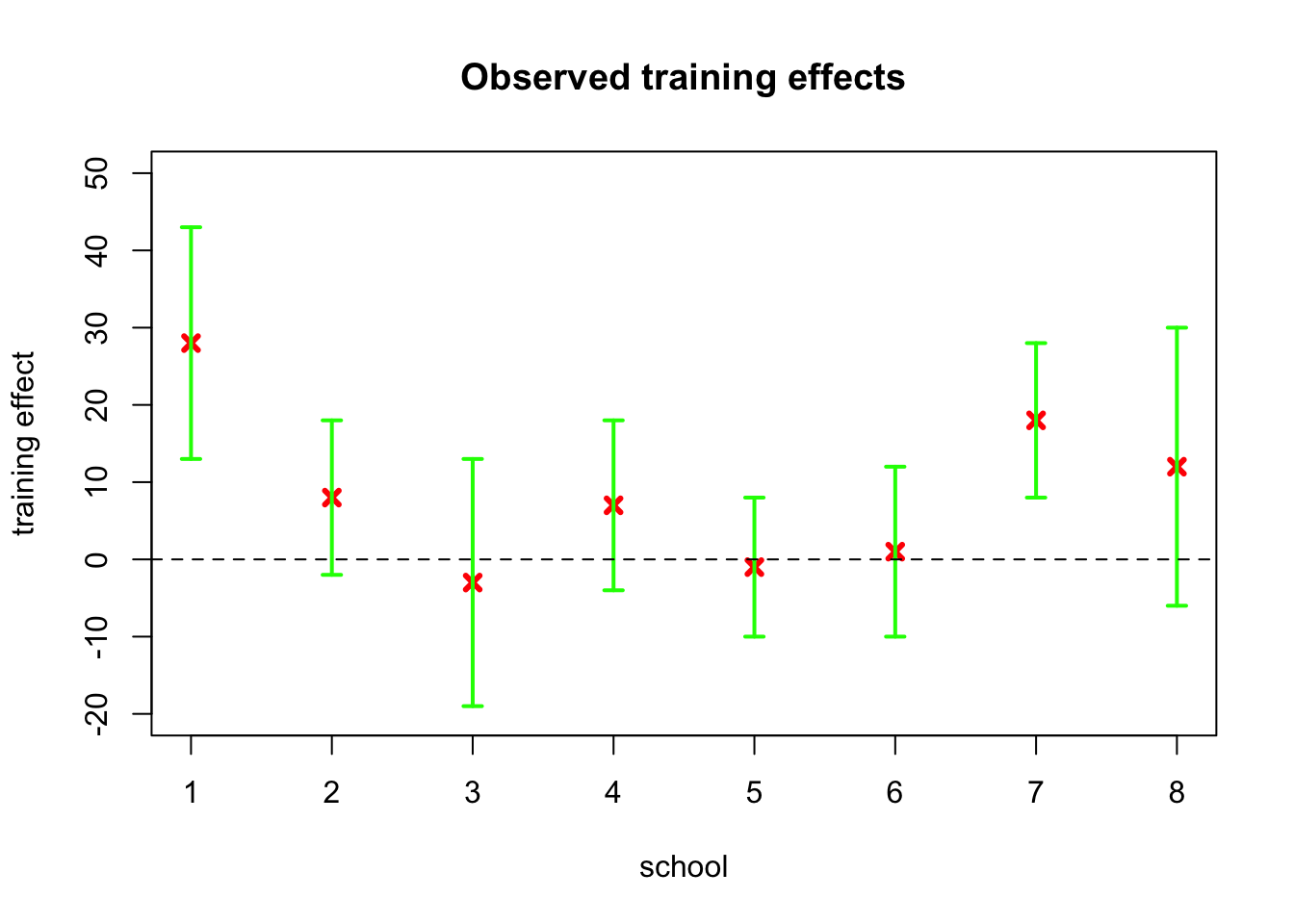

There are clear differences between the schools: for one school the observed training effect is as high as 28 points (normally the test scores are between 200 and 800 with mean of roughly 500 and standard deviation about 100), while for two schools the observed effect is slightly negative. However, the standard errors are also high, and there is substantial overlap between the schools.

Because there are relatively many (> 30) test subjects in each of the schools, we can use the normal approximation for the distribution of the test scores within one school, so that the mean improvement in the training scores can modeled as: \[ \frac{1}{n_j} \sum_{i=1}^{n_j} Y_{ij} \sim N\left(\theta_j, \frac{\hat{\sigma}_j^2}{n_j}\right). \] for each of the \(j = 1, \dots, J\) schools.

To simplify the notation, let’s denote these group means as \(Y_j := \frac{1}{n_j} \sum_{i=1}^{n_j} Y_{ij}\), and the group standard deviations as \(\sigma^2_j := \hat{\sigma}^2_j / n\). Because mean is a sufficient statistic for a normal distribution with a known variance, we can model the sampling distribution with only one observation from each of the schools: \[ Y_j \,|\,\theta_j \sim N(\theta_j, \sigma^2_j) \quad \text{for all} \,\, j = 1, \dots, J \] using the notation defined above.

Furthermore, we assume that the true training effects \(\theta_1, \dots, \theta_J\) for each school are a sample from the common normal distribution¹²: \[ \theta_j \,|\, \mu, \tau^2 \sim N(\mu, \tau^2) \quad \text{for all} \,\, j = 1, \dots, J. \]

However, before specifying the full hierachical model, let’s first examine two simpler ways to model the data.

6.3.1 No-pooling model

Probably the simplest thing to do would be to assume the true training effects \(\theta_j\) as independent, and use a noninformative improper prior for them: \[ \begin{split} Y_j \,|\,\theta_j &\sim N(\theta_j, \sigma^2_j) \\ p(\theta_j) \,&\propto 1 \quad \text{for all} \,\, j = 1, \dots, J. \end{split} \] Now the joint posterior factorizes: \[ p(\boldsymbol{\theta}|\mathbf{y}) \propto 1 \cdot \prod_{j=1}^J p(y_j| \boldsymbol{\theta}_j), \] which means that the posteriors for the true training effects can be estimated separately for each of the schools: \[ \theta_j \,|\, \mathbf{Y} = \mathbf{y}\sim N(y_j, \sigma_j) \quad \text{for all} \,\, j = 1, \dots, J. \] We have solved the posterior analytically, but let’s also sample from it to draw a boxplot similar to the ones we will produce for the fully hierarchical model:

set.seed(123)
n_sim <- 1e4
theta <- matrix(numeric(n_sim * schools$J), ncol = schools$J)
for(j in 1:schools$J)
  theta[ ,j] <- rnorm(n_sim, schools$y[j], schools$sigma[j])

boxplot(theta, col = 'skyblue', ylim = c(-60, 80), main = 'No pooling model')
abline(h = 0, lty = 2)
points(schools$y, col = 'red', lwd=2, pch=4)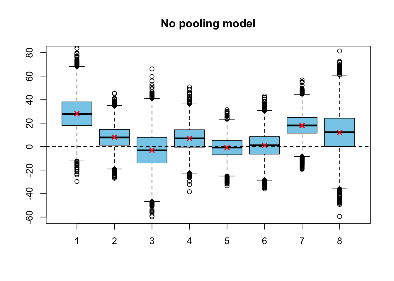

The observed training effects are marked into the figure with red crosses. Because we using a non-informative prior, posterior modes are equal to the observed mean effects. It seems that by using the separate parameter for each of the schools without any smoothing we are most likely overfitting (we will actually see if this is the case at the next week!). Notice that if we used a noninformative prior, there actually would be some smoothing, but it would have been into the direction of the mean of the arbitrarily chosen prior distribution, not towards the common mean of the observations. Setting the arbitrary noninformative prior would make very little sense here, because we can actually use the values of the other groups to infer the parameters of this prior distribution (which is called a population distribution in the full hierarchical model).

6.3.2 Complete pooling model

But before we examine the full hierarchical distribution, let’s try another simplified model. In the so-called complete pooling model we make an apriori assumption that there are no differences between the means of the schools (and probably the standard deviations are also the same; different observed standard deviations are due to different sample sizes and random variance), so that we need only single parameter \(\theta\), which presents the true training effect for all of the schools. Let’s use a noninformative improper prior again: \[ \begin{split} Y_j \,|\, \theta &\sim N(\theta, \sigma^2_j) \quad \text{for all} \,\, j = 1, \dots , J\\ p(\theta) &\propto 1. \end{split} \] We have \(J=8\) observations from the normal distributions with the same mean and different, but known variances. We can derive the posterior for the common true training effect \(\theta\) with a computation almost identical to one performed in Example 5.2.1, in which we derived a posterior for one observation from the normal distribution with known variance: \[ p(\theta|\mathbf{y}) = N\left( \frac{\sum_{j=1}^J \frac{1}{\sigma^2_j} y_j}{\sum_{j=1}^J \frac{1}{\sigma^2_j}},\,\, \frac{1}{\sum_{j=1}^J \frac{1}{\sigma^2_j}} \right) \] The posterior distribution is a normal distribution whose precision is the sum of the sampling precisions, and the mean is a weighted mean of the observations, where the weights are given by the sampling precisions.

Let’s simulate also from this model, and then draw again a boxplot (which is little bit stupid, because exactly the same posterior is drawn eight times, but this is just for the illustration purposes):

pooled_variance <- 1 / sum(1 / schools$sigma^2)
grand_mean <- pooled_variance * sum(schools$y / schools$sigma^2)

theta <- matrix(rnorm(n_sim * schools$J, grand_mean, pooled_variance), 
                ncol = schools$J)

boxplot(theta, col = 'skyblue', ylim = c(-60, 80), main = 'Complete pooling')
abline(h = 0, lty = 2)
points(schools$y, col = 'red', lwd=2, pch=4)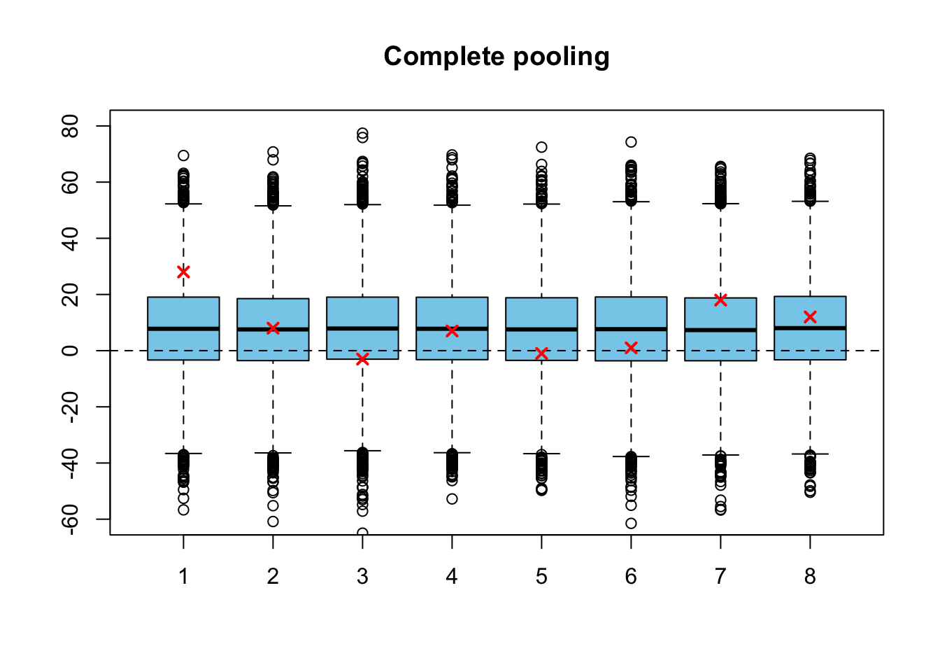

6.3.3 Bayesian hierarchical model

Because the simplifying assumptions of the previous two models do not feel very realistic, let’s also fit a fully Bayesian hierarchical model. To do so we also have to specify a prior to the parameters \(\mu\) and \(\tau\) of the population distribution. It turns out that the improper noninformative prior \[ p(\mu, \tau^2) \propto (\tau^2)^{-1}, \,\, \tau > 0 \] that was used for the normal distribution in Section 5.3 does not actually lead to a proper posterior with this model: with this prior the integral of the unnormalized posterior diverges, so that it cannot be normalized into a probability distribution! However, it turns out that using a completely flat improper prior for the expected value and the standard deviation: \[ p(\mu, \tau) \propto 1, \,\, \tau > 0 \] leads to a proper posterior if the number of groups \(J\) is at least 3 (proof omitted), so we can specify the model as: \[ \begin{split} Y_j \,|\,\theta_j &\sim N(\theta_j, \sigma^2_j) \\ \theta_j \,|\, \mu, \tau &\sim N(\mu, \tau^2) \quad \text{for all} \,\, j = 1, \dots, J \\ p(\mu, \tau) &\propto 1, \,\, \tau > 0. \end{split} \] We can translate this model directly into Stan modelling language:

data {
  int<lower=0> J;
  real y[J];
  real<lower=0> sigma[J];
}

parameters {
  real mu;
  real<lower=0> tau;
  real theta[J];
}

model {
  theta ~ normal(mu, tau);
  y ~ normal(theta, sigma);
}

Notice that we did not explicitly specify any prior for the hyperparameters \(\mu\) and \(\tau\) in Stan code: if we do not give any prior for some of the parameters, Stan automatically assign them uniform prior on the interval in which they are defined. In this case this uniform prior is improper, because these intervals are unbounded.

Now we can sample from this model:

library(rstan)
rstan_options(auto_write = TRUE)
options(mc.cores = parallel::detectCores())

fit3 <- stan('schools1.stan', data = schools, iter = 1e4, chains = 4)

## Warning: There were 415 divergent transitions after warmup. Increasing adapt_delta above 0.8 may help. See
## http://mc-stan.org/misc/warnings.html#divergent-transitions-after-warmup

## Warning: Examine the pairs() plot to diagnose sampling problems

Hmm… Stan warns that there are some divergent transitions: this indicates that there are some problems with the sampling. Stan suggests increasing the tuning parameter adapt_delta from its default value 0.8, so let’s try it before looking at any sampling diagnostics. Values of the adapt_delta are between 0 and 1, and increasing it should decrease the number of divergent transitions while making the sampler slower. Sampling from this simple model is very fast anyway, so we can increase adapt_delta to 0.95. Tuning parameters are given as a named list to the argument control:

fit3 <- stan('schools1.stan', data = schools, iter = 1e4, chains = 4,
             control = list(adapt_delta = 0.95))

## Warning: There were 1015 divergent transitions after warmup. Increasing adapt_delta above 0.95 may help. See
## http://mc-stan.org/misc/warnings.html#divergent-transitions-after-warmup

## Warning: There were 2 chains where the estimated Bayesian Fraction of Missing Information was low. See
## http://mc-stan.org/misc/warnings.html#bfmi-low

## Warning: Examine the pairs() plot to diagnose sampling problems

There are still some divergent transitions, but much less now. If there are lots of divergent transitions, it usually means that the model is specified so that HMC sampling from it is hard¹³, and that the results may be biased because the sampler did not explore the whole area of the posterior distribution efficiently. We will find out later why is it hard for Stan to sample from this model, and how to change the model structure to allow more efficient sampling from the model.

Nevertheless, the proportion of the divergent transitions was not so large when we increased the values of adapt_delta, so we are happy with the results for now. Let’s look at the summary of the Stan fit:

fit3

## Inference for Stan model: schools1.
## 4 chains, each with iter=10000; warmup=5000; thin=1; 
## post-warmup draws per chain=5000, total post-warmup draws=20000.
## 
##            mean se_mean   sd   2.5%    25%    50%    75% 97.5% n_eff Rhat
## mu         8.42    0.27 5.17  -1.87   5.08   8.39  11.97 17.89   368 1.01
## tau        6.23    0.29 5.41   0.51   2.21   4.89   8.67 19.95   358 1.01
## theta[1]  11.62    0.15 7.96  -1.94   6.54  10.90  15.58 30.77  2875 1.00
## theta[2]   8.40    0.27 6.28  -4.53   4.45   8.51  12.74 20.24   539 1.00
## theta[3]   6.82    0.36 7.69 -10.63   2.57   7.41  11.96 19.94   454 1.01
## theta[4]   8.20    0.29 6.53  -5.41   4.17   8.37  12.64 20.45   504 1.01
## theta[5]   5.83    0.40 6.50  -8.45   1.79   6.21  10.35 16.73   258 1.01
## theta[6]   6.76    0.35 6.79  -8.09   2.76   7.14  11.40 18.56   367 1.01
## theta[7]  10.98    0.16 6.65  -1.20   6.65  10.62  14.75 25.69  1765 1.00
## theta[8]   8.90    0.22 7.62  -6.22   4.45   8.81  13.43 25.03  1235 1.00
## lp__     -16.25    0.71 6.82 -27.37 -21.21 -17.39 -11.97 -1.33    91 1.03
## 
## Samples were drawn using NUTS(diag_e) at Wed Mar 13 10:39:29 2019.
## For each parameter, n_eff is a crude measure of effective sample size,
## and Rhat is the potential scale reduction factor on split chains (at 
## convergence, Rhat=1).

We have a posterior distribution for 10 parameters: expected value of the population distribution \(\mu\), standard deviation of the population distribution \(\tau\), and the true training effects \(\theta_1, \dots , \theta_8\) for each of the schools.

Let’s first examine the marginal posterior distributions \(p(\theta_1|\mathbf{y}), \dots p(\theta_8|\mathbf{y})\) of the training effects :

sim3 <- extract(fit3)  

par(mfrow=c(1,1))
boxplot(sim3$theta, col = 'skyblue', main = 'Hierarchical model')
abline(h=0)
points(schools$y, col = 'red', lwd=2, pch=4)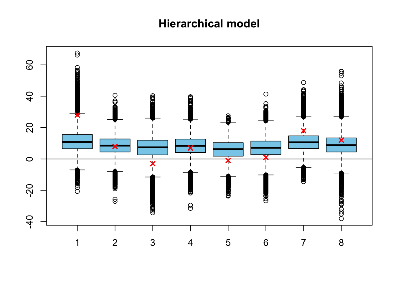

par(mfrow=c(2,4)) 
for(i in 1:8) {
  hist(sim3$theta[,i], col = 'skyblue', main = paste0('School ', i),
       breaks = 30, xlim = c(-20,40), probability = TRUE,
       xlab = bquote(theta[.(i)]))
  abline(v = schools$y[i], lty = 2, lwd = 2, col = 'red')
}

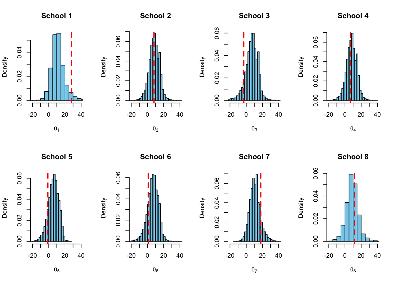
The observed training effects \(y_1, \dots, y_8\) are marked into the boxplot by red crosses, and into the histograms by the red dashed lines. This time the posterior medians (the center lines of the boxplots) are shrunk towards the common mean.

Let’s also take a look at the marginal posteriors of the parameters of the population distribution \(p(\mu|\mathbf{y})\) and \(p(\tau|\mathbf{y})\):

par(mfrow=c(1,2))
hist(sim3$mu, col = 'green', breaks = 30, probability = TRUE,
     main = 'mean', xlab = expression(mu))
abline(v = 0, lty = 2, lwd = 2, col = 'red')
hist(sim3$tau, col = 'red', breaks = 30, probability = TRUE,
     main = 'standard deviation', xlab = expression(tau))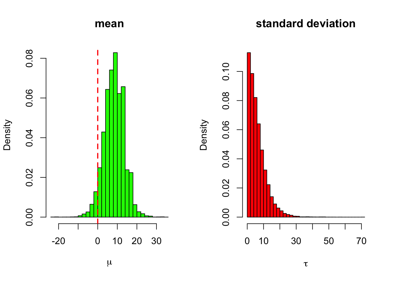

The marginal posterior of the standard deviation is peaked just above the zero. This means that utilizing the empirical Bayes approach here (subsituting the posterior mode or the maximum likelihood estimate for the value of \(\tau\)) in this model would actually lead to radically different results compared to the fully Bayesian approach: because the point estimate \(\hat{\tau}\) for the between-groups variance would be zero or almost zero, the empirical Bayes would in principle reduce to the complete pooling model which assumes that there are no differences between the schools!

6.3.4 Hierarchical model with half-cauchy prior

The original improper prior for the standard devation \(p(\tau) \propto 1\) was chosen out of the computational convenience. Because we are using probabilistic programming tools to fit the model, we do not have to care about the conditional conjugacy anymore, and can use any prior we want. A good choice of prior for the group-level scale parameter in the hierarchical models is a distribution which is peaked at zero, but has a long right tail. Let’s use the Cauchy distribution \(\text{Cauchy}(0, 25)\). The standard deviation of the test scores of the students was around 100, and this could also be thought as an upper limit for the between-the-group variance, so that the realistic interval for \(\tau\) is \((0,100)\). Notice the scale of the \(y\)-axis: this distribution is super flat, but still almost all of its probability mass lies on the interval \((0,100)\). This kind of a relatively flat prior, which is concentrated on the range of the realistic values for the current problem is called a weakly informative prior:

x <- seq(0,100, by = .01)
plot(x, dcauchy(x,0,25), type = 'l', col = 'red', lwd = 2,
     xlab = expression(tau), ylab = 'Density')
legend('topright', 'Cauchy(0,25)', col = 'red', lwd = 2, inset = .1, bty = 'n')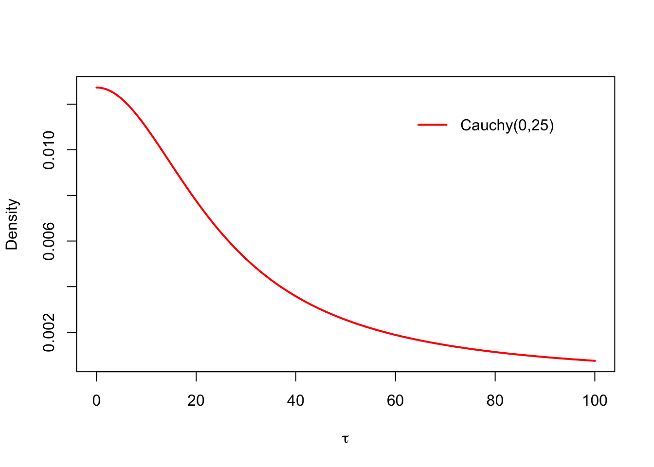

Now the full model is: \[ \begin{split} Y_j \,|\,\theta_j &\sim N(\theta_j, \sigma^2_j) \\ \theta_j \,|\, \mu, \tau &\sim N(\mu, \tau^2) \quad \text{for all} \,\, j = 1, \dots, J \\ p(\mu | \tau) &\propto 1, \,\, \tau \sim \text{half-Cauchy}(0, 25), \,\,\tau > 0. \end{split} \]

The only thing we have to change in the Stan model is to add the half-cauchy prior for \(\tau\):

tau ~ cauchy(0,25);

Because \(\tau\) is constrained into the positive real axis, Stan automatically uses half-cauchy distribution, so above sampling statement is sufficient. Now we can save the whole model into the file schoolsc.stan:

data {
  int<lower=0> J;
  real y[J];
  real<lower=0> sigma[J];
}

parameters {
  real mu;
  real<lower=0> tau;
  real theta[J];
}

model {
  tau ~ cauchy(0,25);
  theta ~ normal(mu, tau);
  y ~ normal(theta, sigma);
}

sim4 <- readRDS('sim7.rds')

Let’s sample from the posterior of this model and examine the results:

## fit4 <- stan('schoolsc.stan', data = schools, iter = 1e4, control = list(adapt_delta = .95))
## sim4 <- extract(fit4)

par(mfrow=c(1,1))
boxplot(sim4$theta, col = 'skyblue',
        main = 'Hierarchical model with Cauchy prior')
abline(h=0)


# compare to medians of model 3 with improper prior for variance
medians3 <- apply(sim3$theta, 2, median)
points(medians3, pch = 4, lwd=2, col = 'green')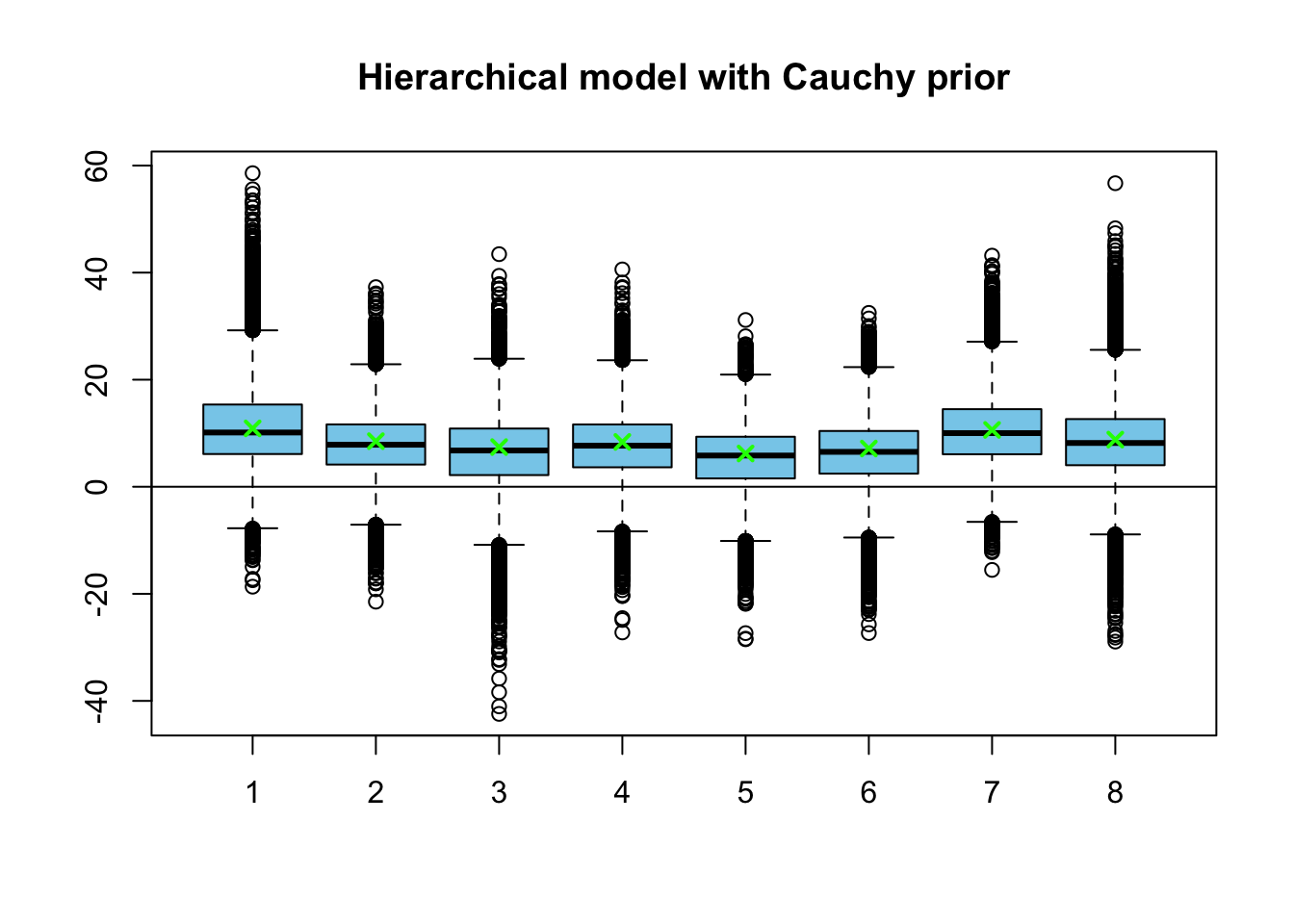

The posterior medians of the hierarchical model are denoted by the green crosses in the boxplot. They match almost exactly the posterior medians for this new model. Let’s also compare the posterior distributions for the group-level variance \(\tau\):

par(mfrow=c(1,2))
hist(sim3$tau, col = 'red', breaks = 30, probability = TRUE,
     main = 'Posterior with uniform prior', xlab = expression(tau),
     ylim =c(0,.12), xlim = c(0,60))
hist(sim4$tau, col = 'red', breaks = 30, probability = TRUE,
     main = 'Posterior with Cauchy(0,25)', xlab = expression(tau),
     ylim =c(0,.12), xlim = c(0,60))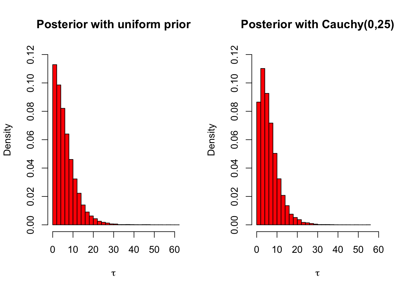

The posteriors for the standard deviation are also almost identical. This is a very good thing: if we want to use a relatively noninformative prior, it is useful to try different priors and prior parameters to see how they affect the posterior. If the posterior is relatively robust with respect to the choice prior, then it is likely that the priors tried really were noninformative. On the other hand, if there are substantial differences between the posterior inferences between the different priors, then at least some of the priors tried were not as noninformative as we believed. This kind of testing the effects of different priors on the posterior distribution is called sensitivity analysis.

6.3.5 Hierarchical model with inverse gamma prior

To perform little bit more ad-hoc sensitivity analysis, let’s test one more prior. The inverse-gamma distribution is a conjugate prior for the variance of the normal distribution¹⁴, so it is a natural choice for a prior. A traditional noninformative, but proper, prior for used for nonhierarchical models is \(\text{Inv-gamma}(\epsilon, \epsilon)\) with some small value of \(\epsilon\); let’s use a smallish value \(\epsilon = 1\) for the illustration purposes. With this prior the full model is: \[ \begin{split} Y_j \,|\,\theta_j &\sim N(\theta_j, \sigma^2_j) \\ \theta_j \,|\, \mu, \tau &\sim N(\mu, \tau^2) \quad \text{for all} \,\, j = 1, \dots, J \\ p(\mu | \tau) &\propto 1, \,\, \tau^2 \sim \text{Inv-gamma}(1, 1). \end{split} \] Notice that we set a prior for the variance \(\tau^2\) of the population distribution instead of the standard deviation \(\tau\). Because of this we declare the variable tau_squared instead of tau in the parameters-block, and declare tau as a square root of tau_squared in the transformed parameters-block:

data {
  int<lower=0> J;
  real y[J];
  real<lower=0> sigma[J];
}

parameters {
  real theta[J];
  real mu;
  real<lower=0> tau_squared;
}

transformed parameters {
  real<lower=0> tau = sqrt(tau_squared);
}

model {
  tau_squared ~ inv_gamma(1,1);
  y ~ normal(theta, sigma);
  theta ~ normal(mu, tau);
}

and then sample from this model:

fit7 <- stan('schoolsig.stan', data = schools, iter = 1e4, 
                           control = list(adapt_delta = .95))

## Warning: There were 49 divergent transitions after warmup. Increasing adapt_delta above 0.95 may help. See
## http://mc-stan.org/misc/warnings.html#divergent-transitions-after-warmup

## Warning: Examine the pairs() plot to diagnose sampling problems

sim7 <- extract(fit7)  

Let’s compare the marginal posterior distributions for each of the schools to the posteriors computed from the hiearchical model with the uniform prior (posterior medians from the model with the uniform prior are marked by green crosses):

par(mfrow=c(1,1))
boxplot(sim7$theta, col = 'skyblue', ylim = c(-20, 40))
abline(h=0)
points(schools$y, col = 'red', lwd=2, pch=4)
points(medians3, pch = 4, lwd=2, col = 'green')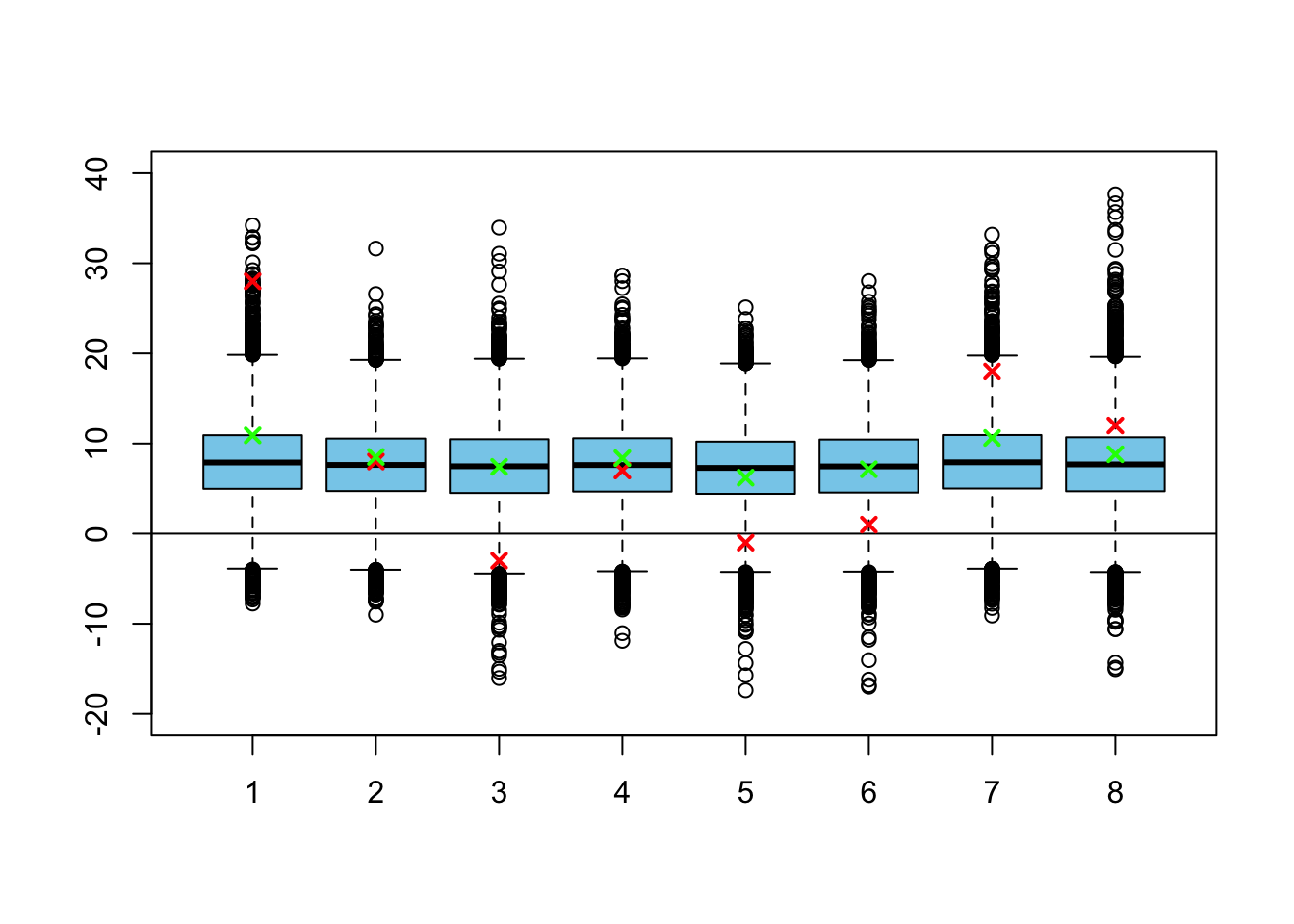

Now the model shrinks the training effects for each of the schools much more! It is almost identical to the complete pooling model. To see why, let’s take a look at the posterior variances:

par(mfrow=c(1,2))
hist(sim3$tau, col = 'red', breaks = 50, probability = TRUE,
     main = 'Improper prior', xlim = c(0,30), xlab = expression(tau))
hist(sim7$tau, col = 'red', breaks = 50, probability = TRUE,
     main = 'Prior Inv-Gamma(1,1)', xlim = c(0,30), xlab = expression(tau))

# multiplied by the jacobian of the inverse transform
dinv_gamma <- function(x,alpha,beta){
  beta^alpha / gamma(alpha) * x^(-2 *(alpha + 1)) * exp(-beta / x^2) * 2 * x  
} 

x <- seq(0, 30, by=.01)
lines(x, dinv_gamma(x, 1, 1), type = 'l', col = 'blue', lwd = 2)
legend('topright', 'Prior', lwd = 2, col = 'blue', inset = .1, bty = 'n')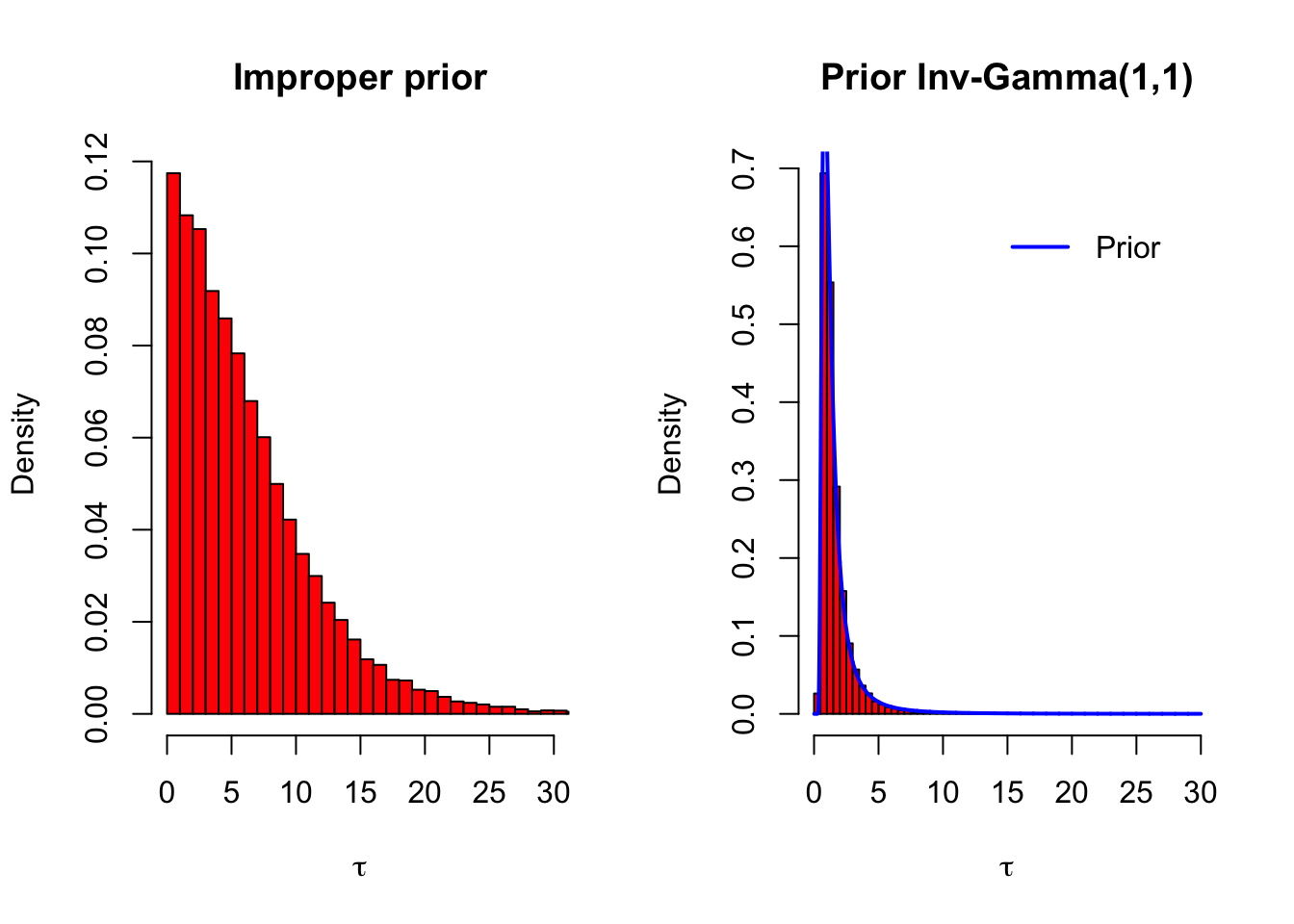

The prior distribution \(\text{Inv-gamma}(1,1)\) (transformed for standard deviation) is drawn on the rigthmost picture with a blue line: it seems that the data had almost no effect at all on the posterior of \(\tau\). So the prior which we thought would be reasonably noninformative, was actually very strong: it pulled the standard deviation of the population distribution to almost zero! This is why performing the sensitivity analysis is important.

References

Murphy, Kevin P. 2012. Machine Learning: A Probabilistic Perspective. Cambridge, MA.

Gelman, A., J.B. Carlin, H.S. Stern, D.B. Dunson, A. Vehtari, and D.B. Rubin. 2013. Bayesian Data Analysis, Third Edition. Chapman & Hall/Crc Texts in Statistical Science. Taylor & Francis. https://books.google.fi/books?id=ZXL6AQAAQBAJ.

---

10. This is why we chose the beta prior for the binomial likelihood in Problem 4 of Exercise set 3, in which we estimated the proportions of the very liberals in each of the states.↩

11. Actually this assumption was made to simplify the analytical computations. Since we are using proabilistic programming tools to fit the model, this assumption is no longer necessary. But because we do not have the original data, and it this simplifying assumption likely have very little effect on the results, we will stick to it anyway.↩

12. By using the normal population distribution the model becomes conditionally conjugate. Now that we are using Stan to fit the model, also this assumption is no longer necessary.↩

13. Or it may mean that the model was specified completely wrong: for instance, some of the parameter constraints may be forgotten. This is a first thing that should be checked if there are lots of divergent transitions.↩

14. Remember that the inverse scaled chi squared distribution we used is just an inverse-gamma distribution with a convenient reparametrization.↩