Chapter 5 Multiparameter models
We have actually already examined computing the posterior distribution for the multiparameter model because we have made an assumption that the parameter \(\boldsymbol{\theta} = (\theta_1, \dots, \theta_d)\) is a \(d\)-component vector, and examined one-dimensional parameter \(\theta\) as a special case of this.
For instance, in the exercises we computed a posterior distribution for the parameter \(\boldsymbol{\theta}\) of the multinomial distribution \(\text{Multinom}(n, \boldsymbol{\theta})\). We were interested in the values of the whole parameter vector \(\boldsymbol{\theta} = (\theta_1, \dots, \theta_d)\): this means that the full posterior distribution \(p(\boldsymbol{\theta}|\mathbf{y})\) was the desired result. This situation did not in principle differ from the one-dimensional case.
However, often we are not interested in the full posterior \(p(\boldsymbol{\theta}|\mathbf{y})\), but only in the marginal posterior distributions of some of the components of the parameter vector.
A classical example is a case in which we are interested in measuring some quantity, for example the speed of light, and model our measurements \(Y_1, \dots, Y_n\) of the value of this quantity as an independent sample from the normal distribution: \[ Y_i \sim N(\mu, \sigma^2) \quad \text{for all} \,\, i = 1, \dots ,n. \] Now the parameter \(\boldsymbol{\theta} = (\mu, \sigma^2)\) of the model is two-dimensional, but sometimes we are only interested in the true value of the quantity \(\mu\), and not so much on our measurement error \(\sigma^2\). The parameter \(\sigma^2\) is called a nuisance parameter here.
More generally, we will consider a situation in which the parameter vector \(\boldsymbol{\theta} = (\boldsymbol{\theta}_1, \boldsymbol{\theta}_2)\) is partitioned into two (possibly also vector-valued) components, \(\boldsymbol{\theta}_1\) being the parameter of interest, and \(\boldsymbol{\theta}_2\) being the nuisance parameter.
5.1 Marginal posterior distribution
Assume the partition of the parameter vector into two components: \(\boldsymbol{\theta} = (\boldsymbol{\theta}_1, \boldsymbol{\theta}_2)\). A distribution \(p(\boldsymbol{\theta}_1|\mathbf{y})\) of the parameter of interest7 given the data is called a marginal posterior distribution, and it can be computed by integrating the nuisance parameter out of the full posterior distribution: \[ p(\boldsymbol{\theta}_1|\mathbf{y}) = \int p(\boldsymbol{\theta}|\mathbf{y})\,\text{d} \boldsymbol{\theta}_2 \] This integral can also be written as \[ \begin{split} p(\boldsymbol{\theta}_1|\mathbf{y}) &= \int p(\boldsymbol{\theta}_1, \boldsymbol{\theta}_2|\mathbf{y})\,\text{d} \boldsymbol{\theta}_2 \\ &= \int p(\boldsymbol{\theta}_1| \boldsymbol{\theta}_2, \mathbf{y}) p(\boldsymbol{\theta}_2|\mathbf{y}) \,\text{d} \boldsymbol{\theta}_2. \end{split} \] A distribution \(p(\boldsymbol{\theta}_1| \boldsymbol{\theta}_2, \mathbf{y})\) is called a conditional posterior distribution of the parameter \(\boldsymbol{\theta}_1\); the above integral can be seen as an weighted average of the conditional posterior distribution, where the weights are given by the marginal posterior distribution of the nuisance parameter \(\boldsymbol{\theta}_2\).
5.2 Inference for the normal distribution with known variance
The normal distribution is ubiquitous in the statistics and machine learning models, and it is also a nice example of the multiparameter inference, because its parameter is two-dimensional \(\boldsymbol{\theta} = (\theta, \sigma^2)\), where often (but not always) an expected value \(\theta\) is considered a parameter of interest, and a variance \(\sigma^2\) is considered a nuisance parameter. Thus, we will go through the posterior inference for the normal model distribution here as an example of the multiparameter inference.
However, before going to the actual multiparameter inference, we will consider a simpler example where we assume the variance \(\sigma^2_0\) of the normal distribution fixed. This is actually an example of the one-parameter conjugate model, because the only unknown parameter is the expected value \(\theta\) of the distribution.
The posterior distribution for the inverse case in which the expected value is assumed to be known, but the variance is unknown, was derived in the exercises. These simple models in which one of the parameters is fixed are useful for deriving the conditional posterior distributions in the case where both the mean and variance are unknown.
5.2.1 One observation
Assume first that we have one observation \(Y\) from the normal distribution with an unknown mean \(\theta\) and a fixed variance \(\sigma^2_0 > 0\). A conjugate distribution for this model is a normal distribution, so that the full model is: \[ \begin{split} Y &\sim N(\theta,\sigma_0^2) \\ \theta &\sim N(\mu_0, \tau_0). \end{split} \] The likelihood of this model can be written as \[ p(y|\theta) = \frac{1}{\sqrt{2\pi\sigma^2_0}} \exp\ \left(-\frac{(y-\theta)^2}{2\sigma^2_0}\right) \propto \exp\ \left(-\frac{\theta^2 - 2y\theta}{2\sigma^2_0}\right), \] and the prior distribution as \[ p(\theta) = \frac{1}{\sqrt{2\pi\tau^2_0}} \exp \left( - \frac{(\theta - \mu_0)^2}{2\tau_0^2} \right) \propto \exp \left( -\frac{\theta^2 - 2\mu_0\theta}{2\tau_0^2} \right). \]
In both the likelihood and the prior the term in the exponent is a quadratic function of the parameter \(\theta\), so this looks promising: we only have to recognize the same quadratic form of \(\theta\) from the posterior to see that it is a normal distribution. Let’s write the unnormalized posterior using the Bayes formula to find out the parameters of the posterior distribution: \[ \begin{split} p(\theta | y) &\propto p(y|\theta)p(\theta) \\ &\propto \exp \left(-\frac{\theta^2 - 2\mu_0\theta}{2\tau_0^2} -\frac{\theta^2 - 2y\theta}{2\sigma^2_0}\right) \\ &= \exp \left( - \frac{\sigma_0^2 (\theta^2 - 2\mu_0\theta) + \tau_0^2(\theta^2 - 2y\theta)}{2\tau_0^2\sigma_0^2} \right) \\ &\propto \exp \left( - \frac{(\sigma_0^2 + \tau_0^2)\theta^2 - 2(\sigma_0^2\mu_0 + \tau_0^2y)\theta}{2\tau_0^2\sigma_0^2} \right)\\ &\propto \exp \left(-\frac{\theta^2 - 2\mu_1\theta}{2\tau_1^2} \right), \end{split} \] where \[ \mu_1 = \frac{\sigma_0^2\mu_0 + \tau_0^2y}{\sigma_0^2 + \tau_0^2}, \] and \[ \tau_1^2 = \frac{\tau_0^2\sigma_0^2}{\sigma_0^2 + \tau_0^2}. \] This means that the posterior distribution of the parameter \(\theta\) is the normal distribution \[ \theta \,|\, Y = y \sim N(\mu_1, \tau_1^2). \] We can also write the parameters of the posterior distribution by using the precision, which is an inverse of the variance \(1/\tau^2\). The posterior precision can be written as a sum of the prior precision and the sampling precision (which was assumed to be a known constant): \[ \frac{1}{\tau_1^2} = \frac{1}{\tau_0^2} + \frac{1}{\sigma_0^2}, \] and the posterior mean can be written as a convex combination of the prior mean and the value of the only observation: \[ \mu_1 = \frac{\frac{1}{\tau_0^2}\mu_0 + \frac{1}{\sigma_0^2} y}{\frac{1}{\tau_0^2} + \frac{1}{\sigma_0^2}}, \] where the weights are the prior and the sampling precision.
5.2.2 Many observations
In the previous example we derived the posterior distribution for the normal model with only one observation. But of course usually we have several observations, in which case the full model is: \[ \begin{split} Y_i &\sim N(\theta, \sigma^2) \quad \text{for all} \,\, i = 1, \dots, n,\\ \theta &\sim N(\mu_0, \tau^2). \end{split} \] By repeating the above derivation, this time using the joint likelihood \(p(\mathbf{y}|\theta) = \prod_{i=1}^n p(y_i|\theta)\) instead of the likelihood of the single observation, or by using the previous result and the fact that the mean of the normally distributed random variables has a normal distribution \[ \overline{Y} \sim N(\theta, \sigma^2/n), \] (and that the sample mean \(\overline{y}\) is a so called sufficient statistic for this model) we can see that the posterior is the normal distribution \[ \theta \,|\, \mathbf{Y} = \mathbf{y} \sim N(\mu_n, \tau_n^2), \] where the expected value is \[ \mu_n = \frac{\frac{1}{\tau_0^2}\mu_0 + \frac{n}{\sigma_0^2} \overline{y}}{\frac{1}{\tau_0^2} + \frac{n}{\sigma_0^2}}, \] and the precision is \[ \frac{1}{\tau_n^2} = \frac{1}{\tau_0^2} + \frac{n}{\sigma_0^2}. \] We can again see that the posterior mean is the convex combination of the prior mean and the mean of the observations, and that the weight of the data mean is proportional to the number of observations: the higher the sample size, the stonger the influence of the data on the posterior mean.
5.3 Inference for the normal distribution with noninformative prior
Next we will consider the general case in which have again \(n\) observations from the normal distribution, but this time both the mean \(\mu\) and variance of the distribution are assumed unknown. Using a noninformative improper prior \(1/\sigma^2\) for the parameter \((\mu, \sigma^2)\) our full model is: \[ \begin{split} Y_i &\sim N(\mu, \sigma^2) \quad \text{for all} \,\, i = 1, \dots, n,\\ p(\mu, \sigma^2) &\propto \frac{1}{\sigma^2}. \end{split} \] First we will derive the full posterior distribution of this model, and using this full posterior derive the marginal posteriors for both the expected value \(\mu\) and the variance \(\sigma^2\).
The general conjugate prior for this model is set hierarchically as: \[ \begin{split} \mu\,|\, \sigma^2 &\sim N(\mu_0, \sigma^2 / \kappa_0), \\ \sigma^2 &\sim \text{Inv-}\chi^2 (\nu_0, \sigma^2_0), \end{split} \] so that the joint prior for the parameters is \[ p(\mu, \sigma^2) \propto (\sigma^2)^{-(\nu_0 + 3)/2} \exp \left\{ - \frac{\nu_0 \sigma_0^2 + \kappa_0 (\mu_0 - \mu)^2}{2 \sigma^2} \right\}. \] This distribution is called the normal inverse chi-squared distribution (NIX) and denoted as \[ (\mu, \sigma^2) \sim N\text{-Inv-}\chi^2(\mu_0, \sigma_0^2 / \kappa_0, \nu_0, \sigma_0^2). \] We will show in the exercises that the full posterior distribution for the parameter \((\mu, \sigma^2)\) is also of this form, but let’s first solve the joint posterior and the marginal posteriors in the special case of noninformative prior.
5.3.1 Full posterior
By using the following factorization (this can be easily proven by writing the left hand side out and rearranging terms): \[ \sum_{i=1}^n (y_i - \mu)^2 = \sum_{i=1}^n (y_i - \bar{y})^2 + n(\bar{y} - \mu)^2, \] and the likelihood for \(n\) independent observations from the same normal distribution: \[ p(\mathbf{y}|\mu, \sigma^2) = \prod_{i=1}^j p(y_i|\mu, \sigma^2) \propto \sigma^{-n} \exp \left\{ - \frac{\sum_{i=1}^n (y_i - \mu)^2}{2\sigma^2} \right\} \] we can write the unnormalized join posterior distribution of both \(\mu\) and \(\sigma^2\) as: \[ \begin{split} p(\mu, \sigma^2 | \mathbf{y}) &\propto p(\mu, \sigma^2) p(\mathbf{y} | \mu, \sigma^2) \\ &\propto \sigma^{-2} \cdot \sigma^{-n} \exp \left\{ - \frac{\sum_{i=1}^n (y_i - \mu)^2}{2\sigma^2} \right\} \\ &\propto \sigma^{-n-2} \exp \left\{ - \frac{\sum_{i=1}^n (y_i - \bar{y})^2 + n(\bar{y} - \mu)^2}{2\sigma^2} \right\} \\ &\propto \sigma^{-n-2} \exp \left\{ - \frac{(n-1)s^2 + n(\bar{y} - \mu)^2}{2\sigma^2} \right\}, \\ \end{split} \] where the sample mean \[ \bar{y} = \frac{1}{n} \sum_{i=1}^n y_i \] and the sample variance \[ s^2 = \frac{1}{n-1} \sum_{i=1}^n (y_i - \bar{y})^2 \] form a two-dimensional sufficient statistics \((\overline{y}, s^2)\) for the parameter \((\mu, \sigma^2)\).
This is a special case of the so-called normal inverse chi-squared distribution, which is a two-dimensional four-parameter distribution. To make this a little bit more concrete, we will generate a sample of 25 points from a standard normal distribution \(N(0,1)\), and plot (unnormalized) full posterior distributions for the first 2, 5, 10 and 25 points. Notice that because we use noninformative prior, the results are not very stable: the posterior for the first two observations is drastically different depending on the values of the observations. You can verify this by running the code without setting the random seed or using different values for the seed. However, with a sample size of \(n=25\) the posterior starts to concentrate on the neigbhorhood of the parameter value \((\mu,\sigma^2) =(0,1)\) of the true generating distribution:
set.seed(0)

q <- function(mu, sigma_squared, m_0, kappa_0, nu_0, sigma_squared_0) {
  (1 / sigma_squared)^(nu_0 + 3 / 2) *
    exp(-(nu_0 * sigma_squared_0 + kappa_0 * (mu - m_0)^2) / (2 * sigma_squared))
}

persp_NI <- function(m_0, kappa_0, nu_0, sigma_squared_0,
                     xlim = c(-1.5,1.5), ylim = c(0,2), grid_incr = .05, ...)  {
  grid_1 <- seq(-1.5, 1.5, by = grid_incr)
  grid_2 <- seq(0.01,2, by = grid_incr)
  grid_2d <- expand.grid(grid_1, grid_2)

  grid_density <- q(grid_2d[ ,1], grid_2d[ ,2], m_0, kappa_0, nu_0, sigma_squared_0)
  head(grid_density)
  grid_matrix1 <- matrix(grid_density / sum(grid_density), nrow = length(grid_1))

  persp(grid_1, grid_2, grid_matrix1, xlim = xlim, ylim = ylim, theta = -45, phi = 30,
        xlab = 'mean', ylab = 'variance', zlab = 'Density', ...)
}

persp_posterior <- function(y, mu_0, kappa_0, nu_0, sigma_squared_0) {
  print(y)
  n <- length(y)
  mu_n <- (kappa_0 * mu_0 + n * mean(y)) / (kappa_0 + n)
  kappa_n <- kappa_0 + n
  nu_n <- nu_0 + n
  sigma_squared_n <- (nu_0 * sigma_squared_0 + (n-1) * var(y) + (kappa_0 * n) /
                        (kappa_0 + n) * (mean(y) - mu_0)^2) / nu_n
  persp_NI(mu_n, kappa_n, nu_n, sigma_squared_n)
}

S <- 100
y <- sample(rnorm(S))
par(mfrow = c(2,2), mar = c(0,0,2,2))
n_stops <- c(2,5,10,25)

for(n in n_stops) {
  y_crnt <- y[1:n]
  cat('n =', n, ', mean =', round(mean(y_crnt), 2),
      ', variance =', round(var(y_crnt), 2), '\n\n')
  persp_NI(m_0 = mean(y_crnt), kappa_0 = n, nu_0 = n - 1, sigma_squared_0 = var(y_crnt),
           main = paste('n =', n))
}
## n = 2 , mean = 0.09 , variance = 2## n = 5 , mean = 0.26 , variance = 0.53## n = 10 , mean = 0.37 , variance = 1.09## n = 25 , mean = 0.07 , variance = 0.86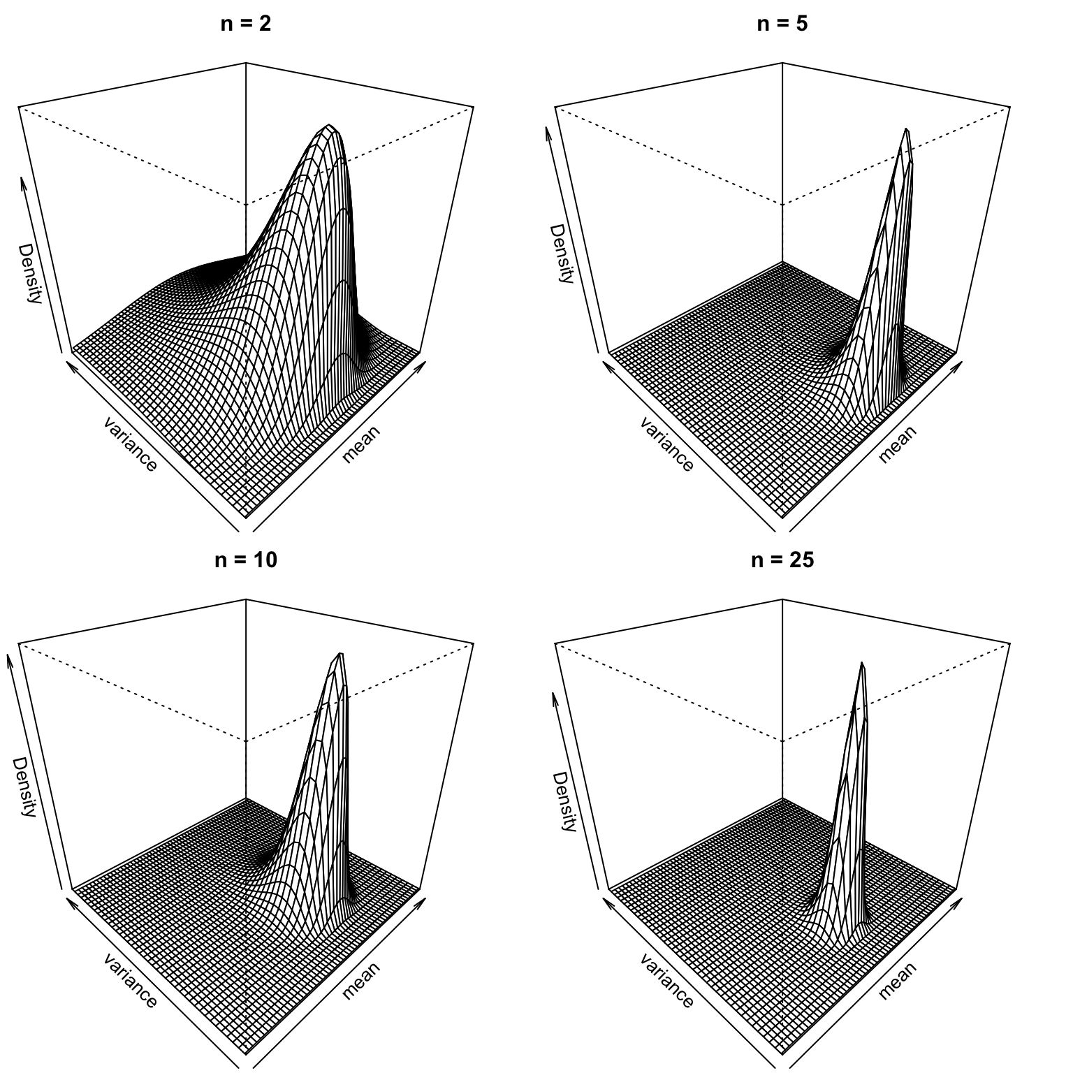
5.3.2 Marginal posterior for the expected value
Assume that the expected value \(\mu\) of the distribution is the parameter of interest and that the variance \(\sigma^2\) is the nuisance parameter. Using the unnormalized joint posterior derived above, we get the marginal posterior of the expected value by integrating it over the variance.
The density of the inverted chi-squared distribution is \[ p(\sigma^2) = \frac{(\nu_0/2)^{\nu_0/2}}{\Gamma(\nu_0/2)} (\sigma_0^2)^{\nu_0/2} (\sigma^2)^{-(\nu_0/2 + 1)} \exp\left(-\frac{\nu_0\sigma_0^2}{2\sigma^2}\right) \quad \text{when} \,\,\sigma^2 > 0, \] and by adding the right constant term we can complete integral into the integral of the inverted chi-squared distribution with parameters \[ \nu_0 := n \] and \[ \sigma^2_0 := (n-1)s^2 / n + (\bar{y} - \mu)^2 \] over its support: \[ \begin{split} p(\mu | \mathbf{y}) &= \int p(\mu, \sigma^2 | \mathbf{y}) \,\text{d} \sigma^2 \\ &\propto \int_0^\infty \sigma^{-n - 2 } \exp \left\{ - \frac{(n-1)s^2 + n(\bar{y} - \mu)^2}{2\sigma^2} \right\} \,\text{d} \sigma^2 \\ &\propto (\sigma_0^2)^{-n/2} \int_0^\infty \frac{(n/2)^{-n/2}}{\Gamma(n/2)}(\sigma_0^2)^{n/2}\, (\sigma^2)^{-\left(\frac{n}{2}+1\right)} \exp \left\{- \frac{n\sigma_0^2}{2\sigma^2} \right\} \,\text{d} \sigma^2 \\ &= \left( (n-1)s^2/n + (\bar{y} - \mu)^2 \right)^{-\frac{n}{2}} \\ &= \left(1 + \frac{1}{(n-1)} \left(\frac{\mu - \bar{y}}{s/\sqrt{n}}\right)^2 \right)^{-\frac{(n-1) + 1}{2}}. \end{split} \] This can be recognized as the kernel of the non-standard \(t\)-distribution with a degree of freedom \(n-1\): \[ \mu \,|\, \mathbf{Y} = \mathbf{y} \sim t_{n-1}(\overline{y}, s^2 / n). \] Thus, the scaled and shifted parameter \(\mu\) follows a standard \(t\) distribution with a degree of freedom \(n-1\): \[ \left. \frac{\mu - \bar{y}}{s/\sqrt{n}} \, \middle| \, \mathbf{Y} = \mathbf{y} \sim t_{n-1} \right.. \] This is an interesting parallel to the result from the classical statstics stating that the so-called \(t\)-statistic, which is a normalized sample mean, has the same distribution8 given the expected value and the variance of the sampling distribution: \[ \left. \frac{\bar{y} - \mu}{s/\sqrt{n}} \, \middle| \, \mu, \sigma^2 \sim t_{n-1} \right.. \]
A \(t\)-distribution has a similar shape than the normal distribution, but it has heavier tails. However, with higher degrees of freedom its shape comes closer to the normal distribution. This behaviour can be seen by standard plotting the densities of standard \(t\)-distributions with different degrees of freedom and comparing them to the density of the standard normal distribution \(N(0,1)\):
x <- seq(-3, 3, by = .01)
n <- c(2,5,10,25)

plot(x, dnorm(x), col = 'violet', lwd = 2, bty = 'n', ylab = 'density', type = 'l')
for(i in seq_along(n))
  lines(x, dt(x, n[i]-1), col = i+1, lwd = 2)
legend('topright', legend = c('N(0,1)', paste('t with df.', n-1)),
       col = c('violet', 2:(length(n)+1)), lwd = 2, bty = 'n')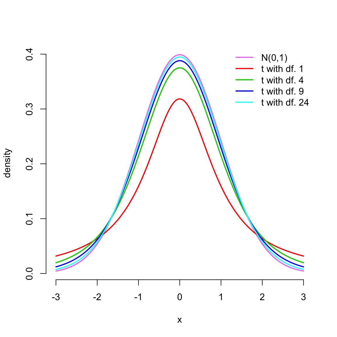
5.3.3 Marginal posterior for the variance
We can also derive the marginal posterior for the variance of the distribution. This time we will utilize the first of the tricks intoduced in Example 1.3.1. The gaussian integral (a.k.a. Euler-Poisson integral): \[ \int_{-\infty}^\infty e^{-x^2} \,\text{d}x= \sqrt{\pi} \] can be evaluated by a transform into the polar coordinates. Also by the change of variables we can see that the gaussian integral of the affine transformation is: \[ \int_{-\infty}^\infty e^{-a(x + b)^2} \,\text{d}x= \sqrt{\frac{\pi}{a}}. \] This is how the normalizing constant of the normal distribution is computed, so we see now that we could have as well used the second of the integrating tricks (completing the integral to the integral of the density function over its support by adding a normalizing constant)9.
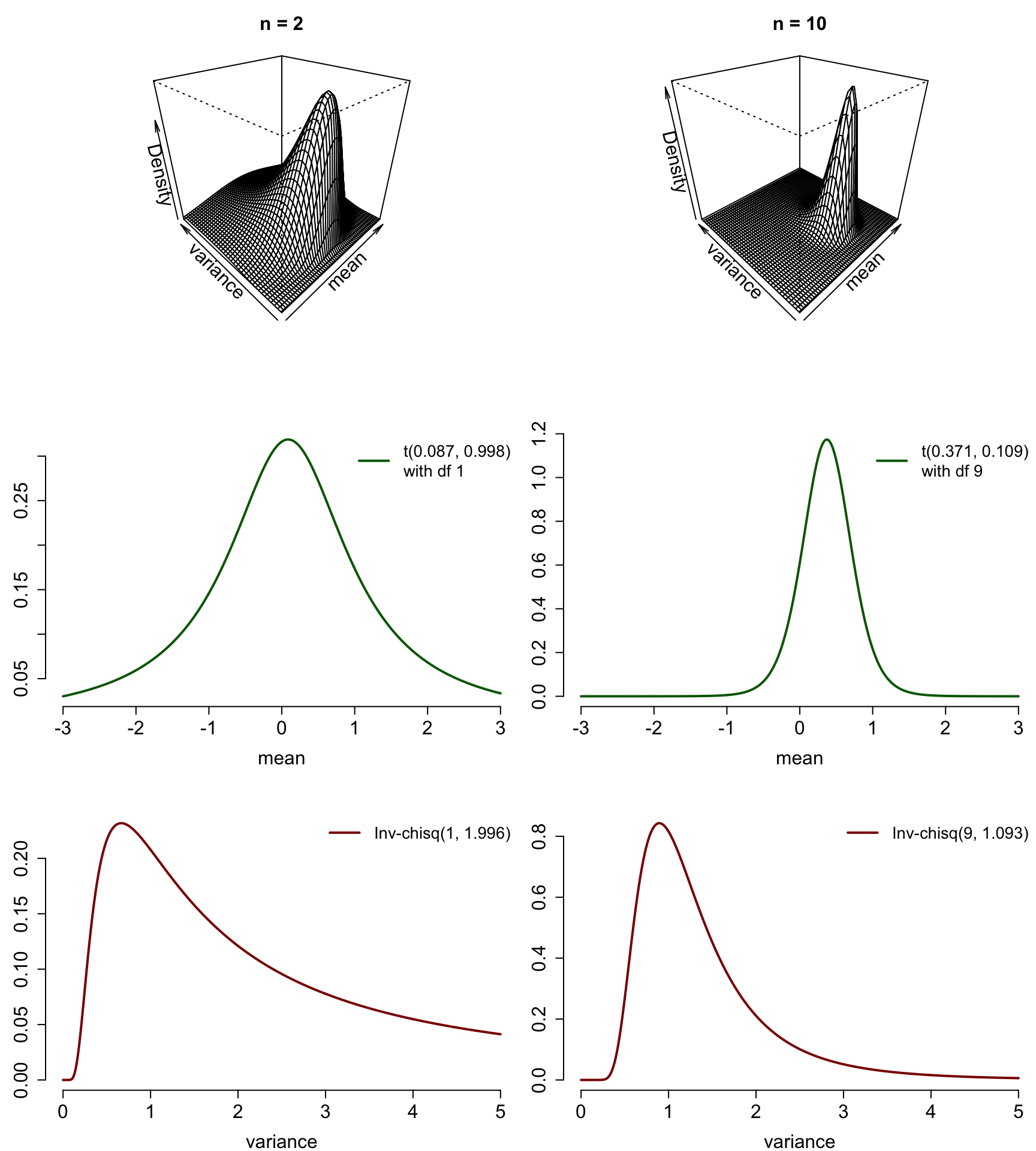
So we get the marginal posterior of the variance \(\sigma^2\) by integrating the expected value \(\mu\) out of the joint posterior distribution: \[ \begin{split} p(\sigma^2|\mathbf{y}) &= \int_{-\infty}^\infty p(\mu, \sigma^2|\mathbf{y}) \, \text{d} \mu \\ &\propto \int_{-\infty}^\infty \sigma^{-n - 2 } \exp \left\{ - \frac{(n-1)s^2 + n(\bar{y} - \mu)^2}{2\sigma^2} \right\} \,\text{d} \mu \\ &= (\sigma^2)^{-n/2 + 1} \exp \left\{ - \frac{(n-1)s^2}{2\sigma^2}\right\} \int_0^\infty \exp \left\{ - \frac{n}{2\sigma^2}(\bar{y} - \mu)^2 \right\} \,\text{d} \mu \\ &= (\sigma^2)^{-n/2 + 1} \exp \left\{ - \frac{(n-1)s^2}{2\sigma^2}\right\} \sqrt{\frac{2\pi\sigma^2}{n}} \\ &\propto (\sigma^2)^{-\left(\frac{n-1}{2} + 1\right)} \exp \left\{ - \frac{(n-1)s^2}{2\sigma^2}\right\}. \end{split} \] This can be regocnized as the kernel of the inverted (scaled) chi-squared distribution with a degree of freedom \(n-1\) and the scale parameter \(s^2\): \[ \sigma^2 \,|\, \mathbf{Y} = \mathbf{y} \sim \chi^{-2}(n-1, \,s^2). \] We can also examine these marginal posteriors we just derived for the parameters \(\mu\) and \(\sigma^2\) visually. In the following are the joint posteriors with a simulated data from \(N(0,1)\), and the corresponding marginal posteriors for the parameters, first with 2, and then with 10 observations:
dnonstandard_t <- function(x, df, mu, sigma_squared) {
  gamma((df + 1) / 2) / (gamma(df / 2) * sqrt(df * pi * sigma_squared)) *
    (1 + 1 / df * (x - mu)^2 / sigma_squared)^(-(df + 1) / 2)
}

dinverted_chisq <- function(x, df, sigma_0_squared) {
  ifelse(x > 0, (df / 2)^(df / 2) / gamma(df / 2) * sigma_0_squared^(df / 2) *
    x^(-(df / 2 + 1)) * exp(- df * sigma_0_squared / (2 * x)), 0)
}

n_stops <- c(2,10)
par(mfrow = c(3,2), mar = c(4,3,3,0), cex.lab = 1.5, cex.axis = 1.5,
    cex.sub = 1.5, cex.main = 1.5)

for(n in n_stops) {
  y_crnt <- y[1:n]
  persp_NI(m_0 = mean(y_crnt), kappa_0 = n, nu_0 = n - 1, sigma_squared_0 = var(y_crnt),
           main = paste('n =', n))
}

mu <- seq(-3, 3, by = .01)
for(n in n_stops) {
  y_crnt <- y[1:n]
  plot(x, dnonstandard_t(mu, n-1, mean(y_crnt), var(y_crnt) / n),
       type = 'l', bty = 'n',col = 'darkgreen', lwd = 2, xlab = 'mean', ylab = '')
  legend('topright', legend = paste0('t(', round(mean(y_crnt),3),
         ', ', round(var(y_crnt) / n, 3), ')\nwith df ', n-1),
         col = 'darkgreen', lwd = 2, bty = 'n',  cex = 1.3)
}

sigma_grid <- seq(0,5, by = .01)
for(n in n_stops) {
  y_crnt <- y[1:n]
  plot(sigma_grid, dinverted_chisq(sigma_grid, n-1, var(y_crnt)), ylab = '',
       type = 'l', bty = 'n',col = 'darkred', lwd = 2, xlab = 'variance')
  legend('topright', legend = paste0('Inv-chisq(', n-1, ', ',
         round(var(y_crnt), 3), ')'), col = 'darkred', lwd = 2, bty = 'n', cex = 1.3)
}
Here we refer to \(\boldsymbol{\theta}_1\) as the parameter of interest and to \(\boldsymbol{\theta}_2\) as the nuisance parameter because of the clarity of presentation, but of course \(\boldsymbol{\theta} = (\boldsymbol{\theta}_1, \boldsymbol{\theta}_2)\) can be any partition of the parameter vector.↩
This result holds exactly for the observations \(Y_i \sim N(\mu, \sigma^2)\) from the normal distribution (the model examined here), and asymptotically otherwise.↩
And more generally, the second of integrating tricks always reduces into this first trick of doing a change of variables to recognize a familiar integral.↩