Chapter 3 Summarizing the posterior distribution
In principle, the posterior distribution contains all the information about the possible parameter values. In practice, we must also present the posterior distribution somehow. If the examined parameter \(\theta\) is one- or two dimensional, we can simply plot the posterior distribution. Or when we use simulation to obtain values from the posterior, we can draw a histogram or scatterplot of the simulated values from the posterior distribution. If the parameter vector has more than two dimensions, we can plot the marginal posterior distributions of the parameters of interest.
However, we often also want to summarize the posterior distribution numerically. The usual summary statistics, such as the mean, median, mode, variance, standard devation and different quantiles, that are used to summarize probability distributions, can be used. These summary statistics are often also easier to present and interpret than the full posterior distribution.
3.1 Credible intervals
Credible interval is a “Bayesian confidence interval”. But unlike frequentist confidence intervals, credible intervals have a very intuitive interpretation: it turns out that we can actually say 95% credible interval actually contains a true parameter value with 95% probability! Let’s first define as credible interval more rigorously, and then examine the most common ways to choose the credible intervals.
3.1.1 Credible interval definition
For one-dimensional parameter \(\Theta \in \Omega\) (in this section we will also assume that the parameter is continuous, because it makes no sense to talk about the credible intervals for the discrete parameter), and confidence level \(\alpha \in (0,1)\), an interval \(I_\alpha \subseteq \Omega\) which contains a proportion \(1-\alpha\) of the probability mass of the posterior distribution: \[\begin{equation} P(\Theta \in I_\alpha| \mathbf{Y} = \mathbf{y}) = 1 - \alpha, \tag{3.1} \end{equation}\]is called a credible interval2. Usually we talk about a \((1 - \alpha) \cdot 100\)% credible interval; for example, if the confidence level is \(\alpha = 0.05\), we talk about the 95% credible interval.
For the vector-valued \(\Theta \in \Omega \subseteq \mathbb{R}^d\), a (contiguous) region \(I_\alpha \subseteq \Omega\) containing a proportion \(1 - \alpha\) of the probability mass of the posterior distribution: \[ P(\Theta \in I_\alpha| \mathbf{Y} = \mathbf{y}) = 1 - \alpha, \] is called a credible region.
On the definition we conditioned on the observed data, but we can also talk about a credible interval before observing any data. In this case a credible interval means an interval \(I_\alpha\) containing a proportion \(1-\alpha\) of the probability mass of the prior distribution: \[ P(\Theta \in I_\alpha) = 1 - \alpha. \] This may actually be useful if we want to calibrate an informative prior distribution. We may for example have an ad hoc estimate of the region of the parameter space where the true parameter value lies with 95% certainty. Then we just have to find a prior distribution whose 95% credible interval agrees with this estimate. But usually credible intervals are examined after observing the data.
The condition (3.1) does not determine an unique \((1-\alpha) \cdot 100\)% credible interval: actually there is an infinite number of such intervals. This means that we have to define some additional condition for choosing the credible interval. Let’s examine two of the most common extra conditions.
3.1.2 Equal-tailed interval
An equal-tailed interval (also called a central interval) of confidence level \(\alpha\) is an interval \[ I_\alpha = [q_{\alpha / 2}, q_{1 - \alpha / 2}], \] where \(q_z\) is a \(z\)-quantile (remember that we assumed the parameter to be have a continous distribution; this means that the quantiles are always defined) of the posterior distribution.
For instance, 95% equal-tailed interval is an interval \[ I_{0.05} = [q_{0.025}, q_{0.975}], \] where \(q_{0.025}\) and \(q_{0.975}\) are the quantiles of the posterior distribution. This is an interval on whose both right and left side lies 2.5% of the probability mass of the posterior distribution; hence the name equal-tailed interval.
If we can solve the posterior distribution in a closed form, quantiles can be obtained via the quantile function of the posterior distribution: \[ \begin{split} P(\Theta \leq q_z | Y = y) &= z \\ F_{\Theta | \mathbf{Y}}(q_z | y) &= z \\ q_z &= F^{-1}_{\Theta | \mathbf{Y}}(z | y), \end{split} \] This quantile function \(F^{-1}_{\Theta | \mathbf{Y}}\) is an inverse of the cumulative density function (cdf) \(F_{\Theta | \mathbf{Y}}\) of the posterior distribution.
Usually, when a credible interval is mentioned without specifying which type of the credible interval it is, an equal-tailed interval is meant.
However, unless the posterior distribution is unimodal and symmetric, there are point outsed of the equal-tailed credible interval having a higher posterior density than some points of the interval. If we want to choose the credible interval so that this not happen, we can do it by using the highest posterior density criterion for choosing it. We will examine this criterion more closely after an example of equal-tailed credible intervals.
3.1.3 Example of credible intervals
Let’s revisit Example 2.1.1: we have observed a data set \(y=(4, 3, 11, 3 , 6)\), and model it as a Poisson-distributed random vector \(\mathbf{Y}\) using a gamma prior with hyperparameters \(\alpha = 1\), \(\beta = 1\) for the parameter \(\lambda\). Now we want to compute 95% confidence interval for the parameter \(\lambda\).
Let’s first set up our data, hyperparameters and a confidence level:
y <- c(4, 3, 11, 3, 6)
n <- length(y)
alpha <- 1
beta <- 1

alpha_conf <- 0.05
A posterior distribution for the parameter \(\lambda\) is Gamma\((n\overline{y} + \alpha, n + \beta)\). Let’s set up also the parameters of the posterior distribution:
alpha_1 <- sum(y) + alpha
beta_1 <- n + beta
Now we can compute 0.025- and 0.975-quantiles using the quantile function \(F_{\Lambda|\mathbf{Y}}^{-1}\) of the posterior distribution: \[ \begin{split} q_{0.025} &= F^{-1}_{\Lambda | \mathbf{Y}}(0.025 | y) \\ q_{0.975} &= F^{-1}_{\Lambda | \mathbf{Y}}(0.975 | y). \end{split} \]
Luckily R contains a quantile function of the gamma distribution, so we get the 95% credible interval simply as:
q_lower <- qgamma(alpha_conf / 2, alpha_1, beta_1)
q_upper <- qgamma(1 - alpha_conf / 2, alpha_1, beta_1)
c(q_lower, q_upper)
## [1] 3.100966 6.547264Let’s examine this credible interval visually:
lambda <- seq(0,7, by = 0.001) # set up grid for plotting
lambda_true <- 3

plot(lambda, dgamma(lambda, alpha_1, beta_1), type = 'l', lwd = 2, col = 'violet',
     ylim = c(0, 1.5), xlab = expression(lambda),
     ylab = expression(paste('p(', lambda, '|y)')))

y_val <- dgamma(lambda, alpha_1, beta_1)
x_coord <- c(q_lower, lambda[lambda >= q_lower & lambda <= q_upper], q_upper)
y_coord <- c(0, y_val[lambda >= q_lower & lambda <= q_upper], 0)
polygon(x_coord, y_coord, col = 'pink', lwd = 2,  border = 'violet')
abline(v = lambda_true, lty = 2)

lines(lambda, dgamma(lambda, alpha, beta),
      type = 'l', lwd = 2, col = 'orange')
legend('topright', inset = .02, legend = c('prior', 'posterior'),
       col = c('orange', 'violet'), lwd = 2)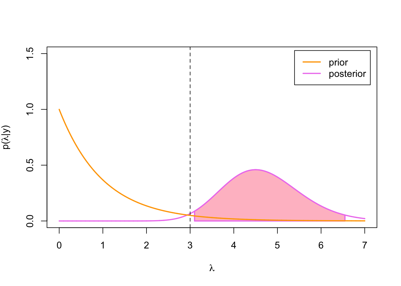
Figure 3.1: 95% equal-tailed CI for Poisson-gamma model
Even though the 95 % credible interval is quite wide because of the low sample size, this time it actually does not contain the true parameter value \(\lambda = 3\) (which we know, because we generated the data from Poisson(3)-distribution!). But let’s see what happens when we increase the sample size:
n_total <- 200
set.seed(111111) # use same seed, so first 5 obs. stay same
y_vec <- rpois(n_total, lambda_true)
head(y_vec)
## [1] 4 3 11 3 6 3n_vec <- c(1, 2, 5, 10, 50, 100, 200)
par(mfrow = c(4,2), mar = c(2, 2, .1, .1))
plot_CI <- function(alpha, beta, y_vec, n_vec, alpha_conf, lambda_true) {
lambda <- seq(0,7, by = 0.01) # set up grid for plotting
plot(lambda, dgamma(lambda, alpha, beta), type = 'l', lwd = 2, col = 'orange',
ylim = c(0, 3.2), xlab = '', ylab = '')
q_lower <- qgamma(alpha_conf / 2, alpha, beta)
q_upper <- qgamma(1 - alpha_conf / 2, alpha, beta)
y_val <- dgamma(lambda, alpha, beta)
polygon(c(q_lower, lambda[lambda >= q_lower & lambda <= q_upper], q_upper),
c(0, y_val[lambda >= q_lower & lambda <= q_upper], 0),
col = 'goldenrod1', lwd = 2, border = 'orange')
abline(v = lambda_true, lty = 2)
text(x = 0.5, y = 2.5, 'prior', cex = 1.75)
for(n_crnt in n_vec) {
y_sum <- sum(y_vec[1:n_crnt])
alpha_1 <- alpha + y_sum
beta_1 <- beta + n_crnt
plot(lambda, dgamma(lambda, alpha_1, beta_1), type = 'l', lwd = 2, col = 'violet',
ylim = c(0, 3.2), xlab = '', ylab = '')
q_lower <- qgamma(alpha_conf / 2, alpha_1, beta_1)
q_upper <- qgamma(1 - alpha_conf / 2, alpha_1, beta_1)
y_val <- dgamma(lambda, alpha_1, beta_1)
x_coord <- c(q_lower, lambda[lambda >= q_lower & lambda <= q_upper], q_upper)
y_coord <- c(0, y_val[lambda >= q_lower & lambda <= q_upper], 0)
polygon(x_coord, y_coord, col = 'pink', lwd = 2, border = 'violet')
lines(lambda, dgamma(lambda, alpha, beta),
type = 'l', lwd = 2, col = 'orange')
abline(v = lambda_true, lty = 2)
text(x = 0.5, y = 2.5, paste0('n=', n_crnt), cex = 1.75)
}
}
plot_CI(alpha, beta, y_vec, n_vec, alpha_conf, lambda_true)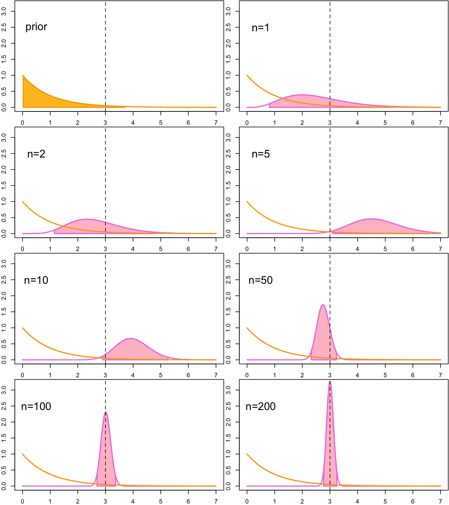 When we observe more data, the credible interval get narrower. This reflects our growing certainty about the range where the true parameter value lies. Turns out that this time the credible interval contains the true parameter value with all the other tested sample sizes expect \(n=5\).
But unlike the frequentist confidence interval, the credible interval does not depend only on the data: the prior distribution also influences the credible intervals. That orange area in the first of the figures is a credible interval that is computed using the prior distribution. It describes our belief where 95% of the probability mass of the distribution should lie before we observe any data.
When we get more observations, credible intervals are influenced more by the the data, and less by the prior distribution. This can be more clearly seen if we use a more strongly peaked prior Gamma\((10,10)\). The expected value of the gamma distributed random variable \(X\) is \[ EX = \frac{\alpha}{\beta}, \] so this prior has a same expected value \(E\lambda = 1\) than the prior Gamma\((1,1)\). But its probability mass is concentrated on much smaller area compared to the relatively flat Gamma\((1,1)\)-prior, so it has a much stronger effect on the posterior inferences:
par(mfrow = c(4,2), mar = c(2, 2, .1, .1))
plot_CI(alpha = 10, beta = 10, y_vec, n_vec, alpha_conf, lambda_true)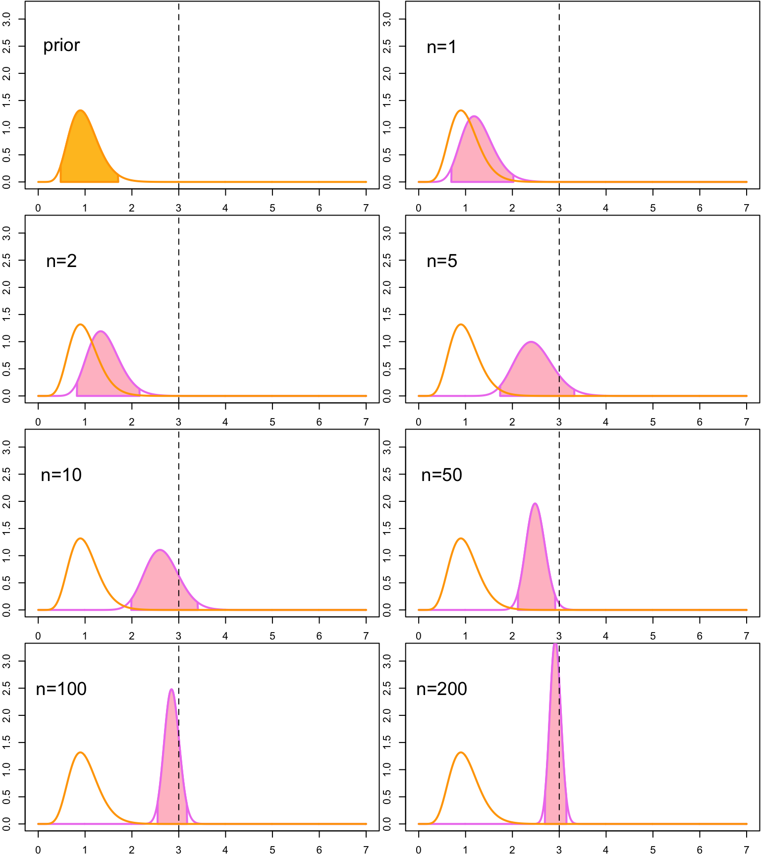
With small sample size the posterior distribution, and thus also the credible intervals, are almost fully determined by the prior; only with the higher sample sizes the data starts to override the effect of the prior distribution on the posterior.
Of course the credible intervals do not have to always be 95% credible intervals. Another widely used credible interval is a 50% credible interval, which contains half of the probability mass of the posterior distribution:
par(mfrow = c(4,2), mar = c(2, 2, .1, .1))
plot_CI(alpha, beta, y_vec, n_vec, alpha_conf = 0.5, lambda_true)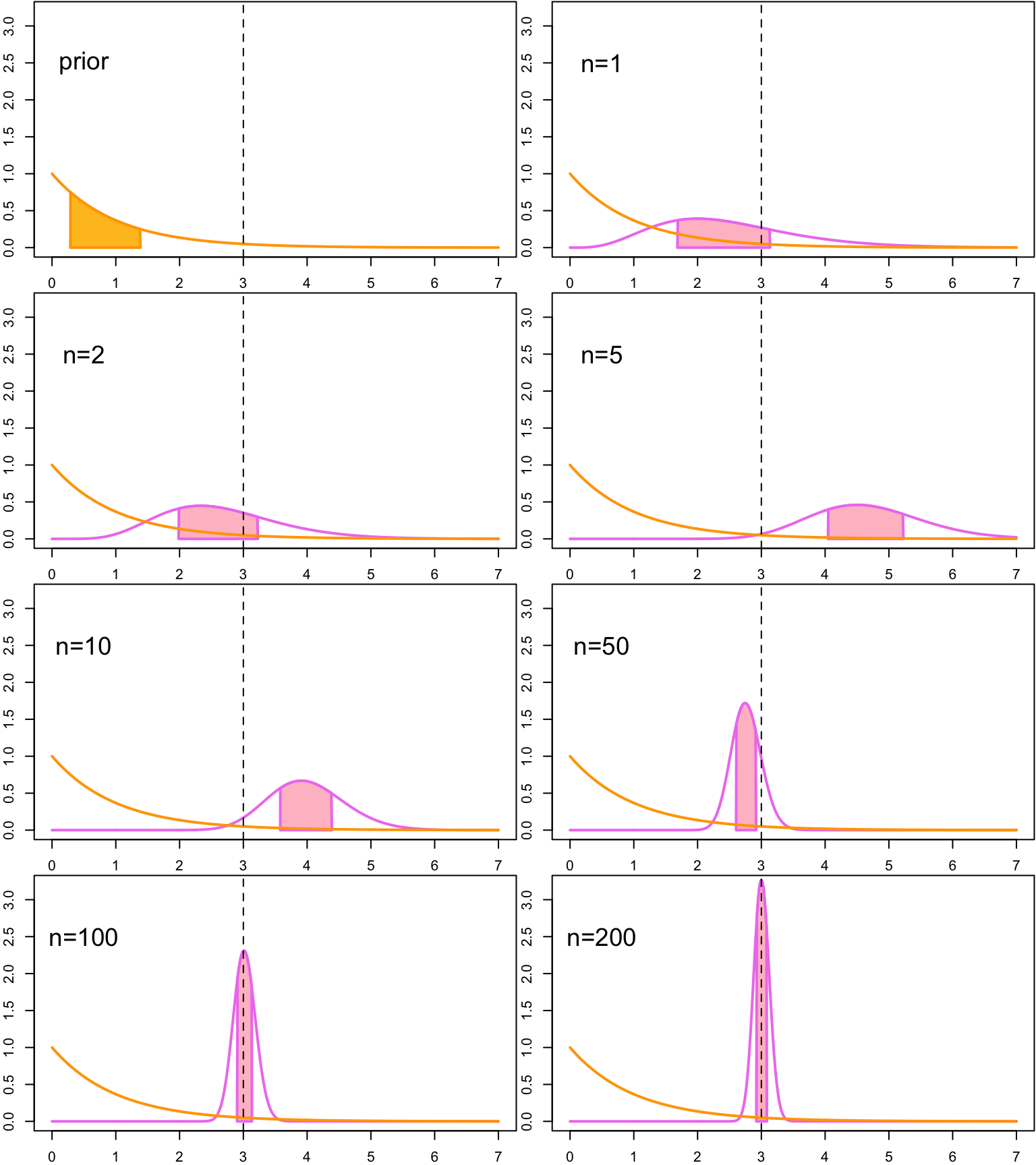
3.1.4 Highest posterior density region
A highest posterior density (HPD) region of confidence level \(\alpha\) is a \((1-\alpha)\)-confidence region \(I_\alpha\) for which holds that the posterior density for every point in this set is higher than the posterior density for any point outside of this set: \[ f_{\boldsymbol{\Theta}|\mathbf{Y}}(\boldsymbol{\theta}|\mathbf{y}) \geq f_{\boldsymbol{\Theta}|\mathbf{Y}}(\boldsymbol{\theta}'|\mathbf{y}) \] for all \(\boldsymbol{\theta} \in I_\alpha\), \(\boldsymbol{\theta}' \notin I_\alpha\). This means that a \((1-\alpha)\)-highest density posterior region is a smallest possible \((1-\alpha)\)-credible region.
An observant reader may notice that the HPD region is not necessarily an interval (or a contiguous region in a higher-dimensional case): if the posterior distribution is multimodal, the HPD region of this distribution may be an union of distinct intervals (or distinct contiguous regions in a higher-dimensional case). This means that HPD regions are not necessarily always strictly credible intervals or regions according to Definition (3.1). However, in Bayesian statistics we often talk simply about HPD intervals, even though may not always be intervals.
Let’s examine a (hypothetical) bimodal posterior density (a mixture of two beta distributions) for which the HPD region is not an interval. An equal-tailed 95% CI is always an interval, even though in this case density values are very low near the saddle point of the density function:
alpha_conf <- .05
alpha_1 <- 11
beta_1 <- 30
alpha_2 <- 25
beta_2 <- 8

mixture_density <- function(x, alpha_1, alpha_2, beta_1, beta_2) {
  .5 * dbeta(x, alpha_1, beta_1) + .5 * dbeta(x, alpha_2, beta_2)
}

# generate data to compute empirical quantiles
n_sim <- 1000000
theta_1 <- rbeta(n_sim / 2, alpha_1, beta_1)
theta_2 <- rbeta(n_sim / 2, alpha_2, beta_2)
theta <- sort(c(theta_1, theta_2))

lower_idx <- round((alpha_conf / 2) * n_sim)
upper_idx <- round((1 - alpha_conf / 2) * n_sim)
q_lower <- theta[lower_idx]
q_upper <- theta[upper_idx]

x <- seq(0,1, by = 0.001)
y_val <- mixture_density(x, alpha_1, alpha_2, beta_1, beta_2)
x_coord <- c(q_lower, x[x >= q_lower & x <= q_upper], q_upper)
y_coord <- c(0, y_val[x >= q_lower & x <= q_upper], 0)

plot(x, mixture_density(x, alpha_1, alpha_2, beta_1, beta_2),
     type='l', col = 'violet', lwd = 2,
     xlab = expression(theta), ylab = 'density')
polygon(x_coord, y_coord, col = 'pink', lwd = 2,  border = 'violet')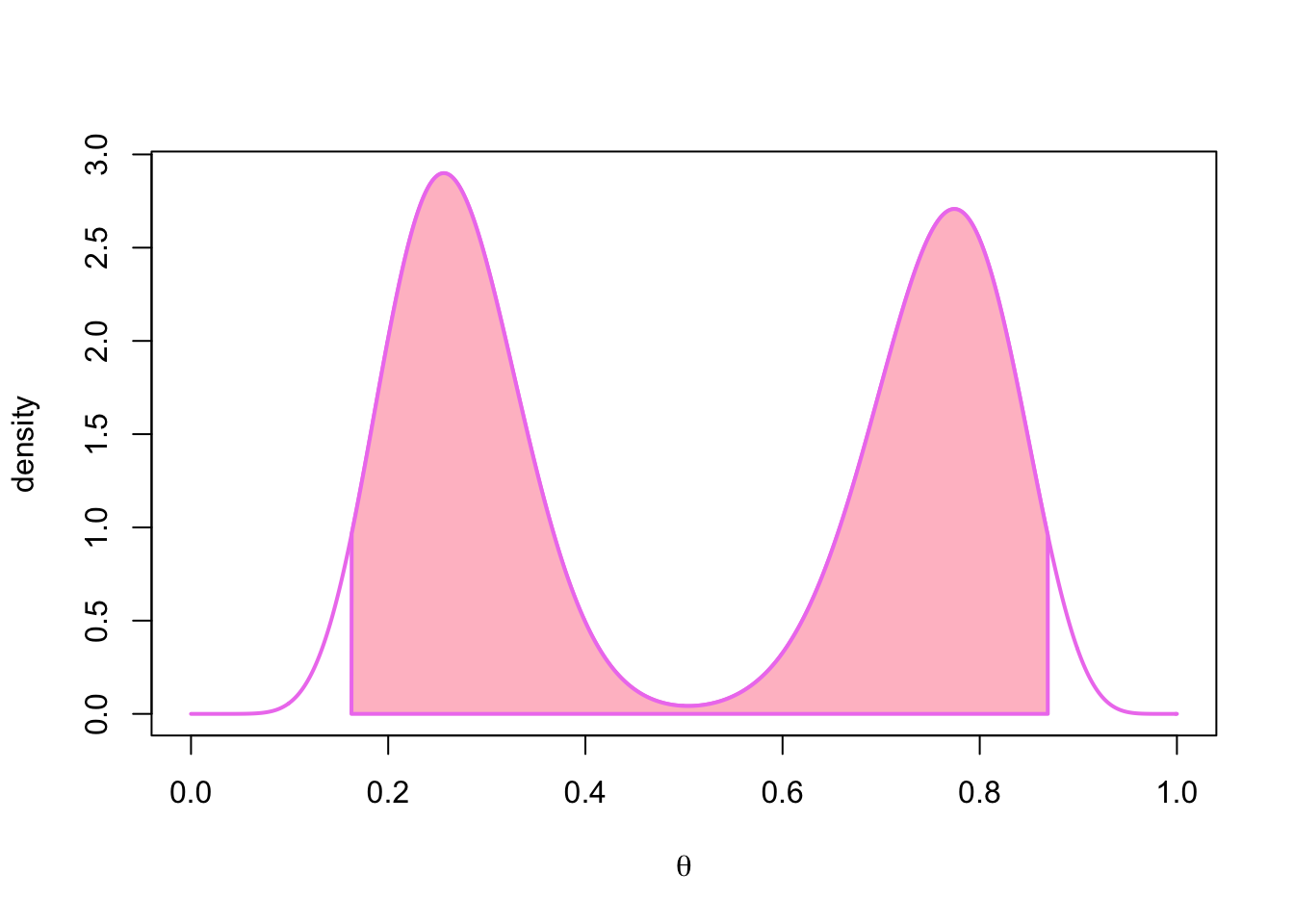
On the other hand a 95% HPD region for this bimodal distribution consists of two distinct intervals:
# install.packages('HDInterval')
dens <- density(theta)
HPD_region <- HDInterval::hdi(dens, allowSplit = TRUE)
height <- attr(HPD_region, 'height')
lower <- HPD_region[1,1]
upper <- HPD_region[1,2]

x_coord <- c(lower, x[x >= lower & x <= upper], upper)
y_coord <- c(0, y_val[x >= lower & x <= upper], 0)

plot(x, mixture_density(x, alpha_1, alpha_2, beta_1, beta_2),
     type='l', col = 'violet', lwd = 2,
     xlab = expression(theta), ylab = 'density')
polygon(x_coord, y_coord, col = 'pink', lwd = 2,  border = 'violet')

lower <- HPD_region[2,1]
upper <- HPD_region[2,2]
x_coord <- c(lower, x[x >= lower & x <= upper], upper)
y_coord <- c(0, y_val[x >= lower & x <= upper], 0)
polygon(x_coord, y_coord, col = 'pink', lwd = 2, border = 'violet')

abline(h = height, col = 'blue', lty = 2, lwd = 2)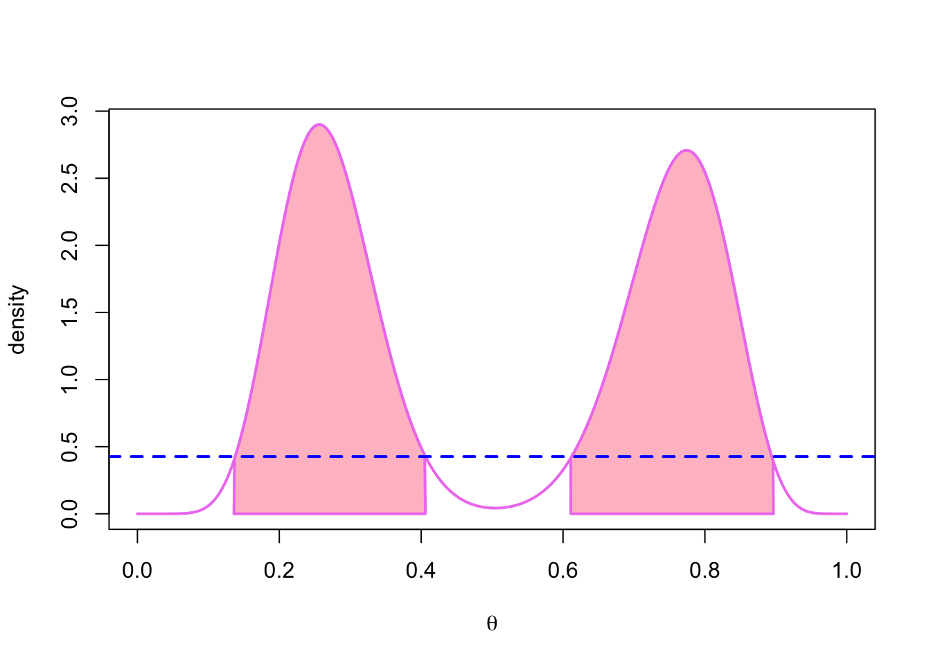
In this case it seems that a highest posterior density region is a better summary of the distribution than the equal-tailed confidence interval. This (imagined) example also demonstrates why it is dangerous to try to reduce the posterior distribution to single summary statistics, such as the mean or the mode of the posterior distribution.
3.2 Posterior mean as a convex combination of means
A mean of the posterior distribution is often also called a Bayes estimator, denoted as \[ \hat{\theta}_\text{Bayes}(Y) := E[\lambda \,|\, \mathbf{Y}]. \]
A mean of the gamma distribution Gamma\((\alpha, \beta)\) is \(\frac{\alpha}{\beta}\), so a posterior mean for the model Poisson-gamma model of Example 2.1.1 is \[\begin{equation} E[\lambda \,|\, \mathbf{Y} = \mathbf{y}] = \frac{\alpha + n\overline{y}}{\beta + n}. \tag{3.2} \end{equation}\]A posterior mean can also be written as a convex combination of the mean of the prior distribution, and the mean of the observations: \[ E[\lambda \,|\, \mathbf{Y} = \mathbf{y}] = \frac{\alpha + n\overline{y}}{\beta + n} = \kappa \frac{\alpha}{\beta} + (1 - \kappa) \overline{y}, \] where the mixing proportion is \[ \kappa = \frac{\beta}{\beta + n}. \] The higher the sample size, the higher is the contribution of the data to the posterior mean (compared to the contribution of the prior mean). And at the limit when \(n \rightarrow \infty\), \(\kappa \rightarrow 0\). This means that for this model the posterior mean is asymptotically equivalent to the maximum likelihood estimator, which for this model is just the mean of the observations: \[ \hat{{\theta}}_\text{MLE}(\mathbf{Y}) = \overline{Y}. \] The formula for the posterior mean of the Poisson-gamma model given in Equation (3.2) also gives us a hint why increasing the rate parameter \(\beta\) of the prior gamma distribution increased the effect of the prior of the posterior distribution: The location parameter \(\alpha\) is added to the sum of the observations, and \(\beta\) is added to the sample size. So the prior could be interpreted as “pseudo-observations” that are added to the actual observations: parameter \(\alpha\) could be interpreted as the “pseudo-events”, and \(\beta\) as the “pseudo-sample size” (although they are not necessarily integers). So using prior \(\alpha = 15\), \(\beta=10\) could be interpreted as having a prior data set of 10 observations, and having total 15 events in this data set.
Remember that we assumed the parameter having a continuous distribution. This means that we can always choose an interval \(I_\alpha\) for which the condition (3.1) holds; we can choose the interval for which the probability is exactly \(1-\alpha\), so we do not have to define the credible interval of having the probability of at least \(1 - \alpha\).↩